The TRANSPOSE Function in Excel: A Comprehensive Overview|2025
/in Advanced Excel Articles /by BesttutorThe TRANSPOSE Function in Excel: Learn how to switch rows and columns for efficient data organization. Master this powerful tool to streamline workflows and enhance productivity!
Excel is a powerful tool used for managing, analyzing, and visualizing data. One of the many features that can greatly enhance productivity is the TRANSPOSE function. This function enables users to switch data from rows to columns or vice versa, offering flexibility in organizing and presenting information. In this paper, we will explore the various aspects of the TRANSPOSE function in Excel, including its use, formulas, shortcuts, and troubleshooting tips. Additionally, we will cover specific scenarios, such as dynamic transposing, transposing based on criteria, and more.
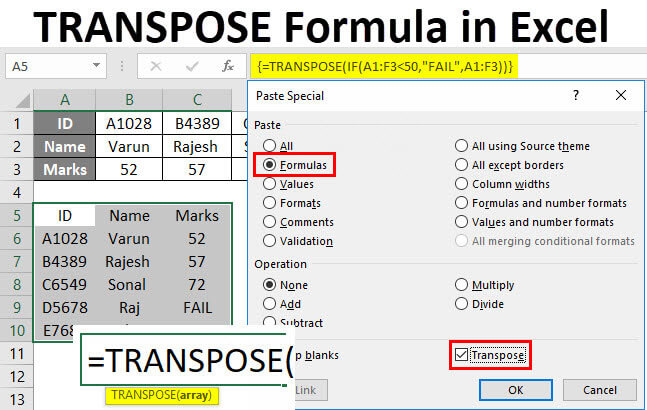
Table of Contents
ToggleIntroduction to the TRANSPOSE Function
The TRANSPOSE function in Excel allows users to swap rows and columns in a data set. This is particularly useful when the arrangement of data needs to be restructured for analysis, reporting, or presentation. Whether you want to turn a horizontal list into a vertical one, or vice versa, the TRANSPOSE function can help.
At its core, the function takes a range of cells (either a row or a column) and rearranges it into the opposite direction, without altering the original data. The general syntax for the TRANSPOSE function is as follows:
=TRANSPOSE(array)
Where array is the range of cells you want to transpose.
Transpose Row to Column in Excel
One of the most common uses of the TRANSPOSE function is to transpose row to column in Excel. This is particularly useful when you have data arranged horizontally, such as a list of months or a sequence of numerical values, and you need to convert it into a vertical format. For instance, if you have the following data in a row:
| January | February | March |
You can use the TRANSPOSE function to convert it into a column format, like this:
| January | | February | | March |
To do this, follow these steps:
- Select the range where you want the transposed data to appear.
- Enter the formula
=TRANSPOSE(A1:C1), whereA1:C1is the range of cells you want to transpose. - Press Ctrl + Shift + Enter (for array formulas) to complete the process.
The data will now appear in a column instead of a row.
Transpose Shortcut in Excel
For users who prefer quick and efficient ways to work within Excel, the transpose shortcut in Excel can be a time-saver. Instead of entering a formula, you can use the following steps to transpose data with a keyboard shortcut:
- Copy the data you wish to transpose (use Ctrl + C).
- Select the destination range where you want to paste the transposed data.
- Right-click the first cell in the destination range.
- Under the Paste Special menu, click Transpose. Alternatively, you can press Alt + E + S + E, followed by Enter.
This method allows you to quickly transpose data without the need for writing a formula.
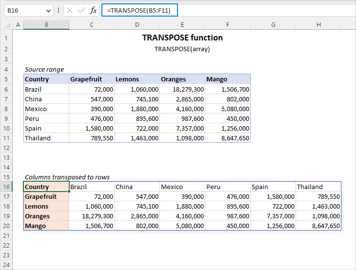
Excel TRANSPOSE Formula Columns to Rows
In some cases, you might need to transpose columns to rows in Excel. This scenario is the inverse of the previous one. If you have a list of vertical data in a column and want to convert it into a horizontal row, the TRANSPOSE function works just as well.
For example, suppose you have the following data in a column:
| 1 | | 2 | | 3 |
To transpose this data into a row, follow these steps:
- Select the destination range where you want to transpose the data.
- Enter the formula
=TRANSPOSE(A1:A3), whereA1:A3represents the range of cells you want to transpose. - Press Ctrl + Shift + Enter (for array formulas).
The data will now appear in a row format:
| 1 | 2 | 3 |
Troubleshooting: Excel TRANSPOSE Function Not Working
While the TRANSPOSE function is generally reliable, there are times when it may not work as expected. Here are a few common reasons for issues:
- Array Formula Errors: The TRANSPOSE function requires array formulas in some cases. If you’re not using Ctrl + Shift + Enter when inputting the formula, Excel may not recognize it as an array formula. To fix this, ensure you are pressing Ctrl + Shift + Enter when entering the formula.
- Mismatched Range Sizes: The range you’re transposing must have the correct number of rows and columns to fit the new layout. For example, if you are transposing a 3×1 range into a row, the destination should be a 1×3 range. If the sizes do not match, Excel will return an error.
- Merged Cells: The presence of merged cells in the source data may prevent the TRANSPOSE function from working correctly. To resolve this, unmerge the cells in the source range before transposing.
- Too Large a Range: If the range of cells you’re trying to transpose is too large, it can result in an error or cause Excel to become unresponsive. If this occurs, try breaking the range into smaller sections.
- Non-Numeric Data: The TRANSPOSE function works with both numeric and non-numeric data, but if there is an issue with a specific type of data (e.g., formulas that reference external workbooks), the function may fail.
How to Convert Vertical to Horizontal in Excel Using Formula
Converting data from vertical to horizontal (or vice versa) can be achieved using the TRANSPOSE function. For example, if you have data arranged in a column and you want to convert it into a row, simply use the following steps:
- Copy the vertical data range (for example,
A1:A5). - Select the range where you want the horizontal data to appear.
- Enter the formula
=TRANSPOSE(A1:A5). - Press Ctrl + Shift + Enter.
This method works when you need to convert data from a vertical list to a horizontal one.
Excel Transpose Multiple Rows in Group to Columns
The Excel transpose multiple rows in group to columns feature is helpful when you need to transpose data in a more complex scenario, such as when you want to group several rows and transpose them into multiple columns.
For instance, suppose you have the following data:
| Name | Age | City |
|---|---|---|
| John | 25 | NY |
| Sara | 30 | LA |
| Mike | 35 | SF |
You can use the TRANSPOSE function to rearrange this data into a set of columns. Here’s how you would do it:
- Select the destination where you want the transposed data.
- Enter the formula
=TRANSPOSE(A1:C3). - Press Ctrl + Shift + Enter.
The result would look something like this:
| Name | John | Sara | Mike |
|---|---|---|---|
| Age | 25 | 30 | 35 |
| City | NY | LA | SF |
This method works well when you need to transpose data with multiple rows and group them into columns.
Dynamic Transpose in Excel
The dynamic transpose in Excel allows you to transpose data that updates automatically when the source data changes. This is a great feature when you want the transposed data to reflect any changes in real-time without having to re-enter the formula.
To set up dynamic transposing, use the TRANSPOSE function in combination with dynamic ranges. For instance, you can use the OFFSET function to create a dynamic range, and then transpose that range. The formula would look something like this:
=TRANSPOSE(OFFSET(A1,0,0,COUNTA(A:A),1))
This formula creates a dynamic range starting from A1 and dynamically adjusts based on the number of rows in column A. The COUNTA(A:A) function counts the non-empty cells in the range and adjusts the number of rows accordingly.

Excel Transpose Rows to Columns Based on Criteria
You can also use the TRANSPOSE function in Excel to transpose rows to columns based on specific criteria. This can be done using IF statements in combination with the TRANSPOSE function. For example, if you have data where certain rows meet specific criteria, and you only want to transpose those rows that meet the condition, you can use an array formula.
For instance, you can use the following formula to transpose data in rows where the value in column A is greater than 10:
=TRANSPOSE(IF(A1:A5>10,B1:B5,""))
This formula will transpose only the values in column B where the corresponding values in column A are greater than 10.
Conclusion
The TRANSPOSE function in Excel is a powerful tool that allows users to manipulate data by changing the orientation of rows and columns. Whether you are looking to convert a row to a column, transpose based on specific criteria, or use shortcuts for quick transposing, the TRANSPOSE function offers flexibility and ease. However, users should be aware of common issues such as array formula errors, merged cells, and large ranges, which can prevent the function from working correctly. By understanding the function’s syntax and how it can be applied in various scenarios, users can make the most of Excel’s capabilities for data manipulation.
GetSPSSHelp is the best choice for mastering the TRANSPOSE function in Excel because of our expert guidance and student-focused approach. Our team simplifies complex concepts, providing clear, step-by-step instructions to help you switch rows and columns effortlessly. We ensure accuracy, save time, and enhance your understanding of Excel. With affordable pricing, 24/7 support, and a commitment to quality, we make learning the TRANSPOSE function stress-free and effective. Whether you’re a beginner or advanced user, GetSPSSHelp empowers you to excel in data analysis. Trust us for reliable, professional assistance that boosts your skills and confidence!
Needs help with similar assignment?
We are available 24x7 to deliver the best services and assignment ready within 3-4 hours? Order a custom-written, plagiarism-free paper
