General instructions:
Select three or more research articles on The History and Evolution of Nursing in Puerto Rico and the United States. (You must include them when submitting the Essay)
Conducts an Essay on The History and Evolution of Nursing in Puerto Rico and the United States and its Influence on the Advances of the Nursing Profession Today.
You must present your writing in double space, in a font Times New Roman, Arial or Courier New, with a font size 12.
Presents 3 pages or more of content. (Does not include cover page and / or references)
Pay attention to grammatical rules (spelling and syntax).
Must be original and should not contain material copied from books or the Internet.
When citing the work of other authors, he presents citations and references using the APA style in order to respect his intellectual property and not incur plagiarism.
Needs help with similar assignment?
We are available 24x7 to deliver the best services and assignment ready within 3-4 hours? Order a custom-written, plagiarism-free paper
Learn how to master the TEXT function in Excel with our comprehensive guide. Understand its syntax, applications, and tips for formatting dates, numbers, and more effectively.
Microsoft Excel is a powerful spreadsheet tool that is used by millions around the world for data analysis, calculations, and presentation. One of the most useful features in Excel is the TEXT function, which allows users to format and manipulate data into a readable text format. In this paper, we will dive into the TEXT function in Excel, explaining how it works, its various applications, and how to use it effectively to improve data analysis and presentation. The paper will also provide examples and the relevant formula formats, making it easy to understand how the TEXT function can be applied in everyday tasks.
What is the TEXT Function in Excel?
The TEXT function in Excel is designed to convert values into text with a specified format. It is commonly used to format dates, times, numbers, and currencies so that they appear in a more user-friendly and readable way. While Excel allows you to perform calculations on numerical data, the TEXT function helps to display the results in a more intuitive or visually appealing manner.
Syntax of the TEXT Function
The syntax for the TEXT function is:
scss
TEXT(value, format_text)
value: This is the numeric value, date, or time that you want to convert into text.
format_text: This is the format that you want to apply to the value. It is typically enclosed in quotation marks (” “), and it specifies how the result should appear.
For instance, if you want to convert a date into a specific format such as “Day-Month-Year,” you would specify that format in the format_text argument.
Why Use the TEXT Function?
There are several practical reasons for using the TEXT function:
Data Presentation: It helps in formatting numbers, dates, or time values so that they are easier to read and understand.
Text Manipulation: It allows the combination of text and numerical values in Excel formulas.
Data Conversion: It provides a way to convert numbers into text, which is useful when preparing data for reports or presentations.
Conditional Formatting: The TEXT function can also be used in conditional formatting to display data with different visual effects based on specific conditions.
In the next sections, we will explore common applications of the TEXT function and its format codes.
Text Functions in Excel with Examples
Formatting Numbers
One of the most common uses of the TEXT function in Excel is formatting numerical data. For instance, if you have a number like 1234567, you can format it as currency or as a number with commas separating thousands.
Example:
scss
=TEXT(1234567, "#,##0")
This formula will convert 1234567 into 1,234,567, with commas separating the thousands.
Another example is formatting a number as currency:
bash
=TEXT(1234.56, "$#,##0.00")
The result will be displayed as $1,234.56, showing the currency symbol and two decimal places.
Formatting Dates
Excel has built-in support for date formatting, and the TEXT function can be used to format dates into various styles. For instance, if you have a date 12/31/2025 in cell A1, you can format it in a different way using the TEXT function.
Example:
scss
=TEXT(A1, "mm/dd/yyyy")
This formula will display the date as 12/31/2025.
Other formats include:
"dddd, mmmm dd, yyyy": Displays Friday, December 31, 2025.
"mmm dd, yyyy": Displays Dec 31, 2025.
Formatting Time
The TEXT function can also be used to format time values. Excel stores time as a fraction of a 24-hour day, so formatting these numbers as times can make them more readable.
For example, if a time is stored as 0.75 (which represents 18:00 or 6 PM), you can display it in a readable format:
scss
=TEXT(0.75, "h:mm AM/PM")
This formula will display 6:00 PM.
Formatting Percentages
If you need to display a number as a percentage, the TEXT function can be used for this purpose as well. For example, converting 0.25 into a percentage:
scss
=TEXT(0.25, "0%")
The result will be 25%. You can also display percentages with decimals:
scss
=TEXT(0.25, "0.00%")
The result will be 25.00%.
Excel TEXT Function Format Codes
The format codes for the TEXT function are used to define how the output will appear. Here are some of the most commonly used format codes:
Number Formatting
0: Displays a digit or 0 if no digit is present (e.g., 001 will display 001).
#: Displays a digit or leaves a space if no digit is present.
,: Adds a thousand separator (e.g., 1234567 becomes 1,234,567).
.: Specifies the decimal point (e.g., 1234.56).
0.0: Rounds the number to one decimal place.
Date and Time Formatting
m: Displays the month as a number (1-12).
mm: Displays the month as a two-digit number (01-12).
mmm: Displays the abbreviated month name (Jan, Feb, etc.).
mmmm: Displays the full month name (January, February, etc.).
d: Displays the day of the month as a number (1-31).
dd: Displays the day of the month as a two-digit number (01-31).
yyyy: Displays the full four-digit year.
h: Displays the hour as a number (1-12 or 0-23 depending on the format).
hh: Displays the hour as a two-digit number (01-12 or 00-23).
mm: Displays the minute as a two-digit number (00-59).
ss: Displays the second as a two-digit number (00-59).
Text Formatting
@: Displays the text as entered (e.g., @ will display the word “Hello” as “Hello”).
These format codes allow you to customize the appearance of numbers, dates, times, and text to meet your specific needs.
How to Use TEXT Function in Excel Formulas
The TEXT function is often used in combination with other Excel functions to perform more complex tasks. One common use is to combine text and numeric values in a single cell.
Combining Text and Formulas in Excel
To combine text and numerical values, you can use the & operator or the CONCATENATE function (although the & operator is recommended in newer versions of Excel). For example, if you want to display a statement like “The total cost is $1234.56”, you can use the following formula:
bash
="The total cost is " & TEXT(1234.56, "$#,##0.00")
This formula will output the result: The total cost is $1,234.56.
Another example:
vbnet
="The current date is " & TEXT(TODAY(), "mmmm dd, yyyy")
This formula will output: The current date is January 31, 2025.
Converting Numbers to Text in Excel
The TEXT function can be used to convert numerical data into text. This is useful in situations where you need to manipulate numbers as text, such as when preparing data for export or generating reports.
For example:
scss
=TEXT(12345, "000000")
This formula will convert 12345 into 012345 by adding leading zeros.
Excel Convert Number to Text Formula
If you want to convert a number into text with a specific format, you can use the following method:
scss
=TEXT(A1, "0.00")
This will convert the number in cell A1 into text with two decimal places.
Conclusion
The TEXT function in Excel is a versatile tool that allows users to convert values into text with custom formatting. It can be used to format numbers, dates, times, and percentages, making data more readable and presentable. Additionally, the TEXT function is invaluable for combining text and numbers in formulas, as well as for converting numerical data into text when needed. By mastering the use of the TEXT function, Excel users can improve the quality of their reports, presentations, and data analysis tasks.
Whether you’re working with large datasets or creating polished presentations, understanding how to use the TEXT function in Excel will enable you to customize and present your data more effectively.
GetSPSSHelp.com stands out as the premier destination for mastering Excel functions, including the TEXT function, thanks to its expert guidance and user-friendly resources. While ExcelJet provides a solid overview of the TEXT function, GetSPSSHelp.com goes further by offering tailored tutorials, practical examples, and step-by-step solutions for real-world scenarios. Their team of experienced professionals ensures that users, from beginners to advanced, can confidently apply the TEXT function to format dates, numbers, and text seamlessly. With personalized support and in-depth explanations, GetSPSSHelp.com is the ultimate choice for anyone seeking to enhance their Excel skills efficiently and effectively.
Needs help with similar assignment?
We are available 24x7 to deliver the best services and assignment ready within 3-4 hours? Order a custom-written, plagiarism-free paper
https://getspsshelp.com/wp-content/uploads/2024/12/logo-8.webp00Besttutorhttps://getspsshelp.com/wp-content/uploads/2024/12/logo-8.webpBesttutor2025-02-01 10:53:442025-09-08 11:09:43Understanding the TEXT Function in Excel|2025
Discover how to use the XLOOKUP function in Excel to perform powerful and flexible lookups. Master this advanced tool for efficient data retrieval and streamlined workflows!
Microsoft Excel is one of the most widely used spreadsheet applications, owing to its powerful functionalities and formulas that allow users to organize, analyze, and manipulate data effectively. Among these formulas, XLOOKUP is one of the most powerful and versatile functions introduced in Excel 365 and Excel 2021. XLOOKUP was designed to replace older lookup functions such as VLOOKUP, HLOOKUP, and LOOKUP, providing a more efficient, flexible, and straightforward way to retrieve data from a range or table. This paper explores the XLOOKUP function in detail, comparing it with VLOOKUP, discussing common issues like XLOOKUP not working, and showcasing examples of how to use XLOOKUP with multiple criteria and across different sheets.
What is XLOOKUP in Excel?
The XLOOKUP function is a modern Excel function that replaces older lookup functions like VLOOKUP and HLOOKUP. It allows users to search for a specific value in a table or range and return a corresponding value from another column or row. XLOOKUP eliminates some of the major limitations of older lookup functions, such as the inability to perform reverse lookups and the restriction on searching only to the right of the lookup value.
Syntax of XLOOKUP Function
The syntax for the XLOOKUP function is as follows:
lookup_value: The value you want to search for in the lookup array.
lookup_array: The range or array that contains the value you want to look up.
return_array: The range or array from which to return the corresponding value.
[if_not_found] (optional): The value to return if the lookup value is not found. By default, XLOOKUP returns an error if the value is not found.
[match_mode] (optional): The match type to use for the lookup. It can be 0 (exact match), -1 (exact match or next smaller item), or 1 (exact match or next larger item).
[search_mode] (optional): The search direction. It can be 1 (search from first to last) or -1 (search from last to first).
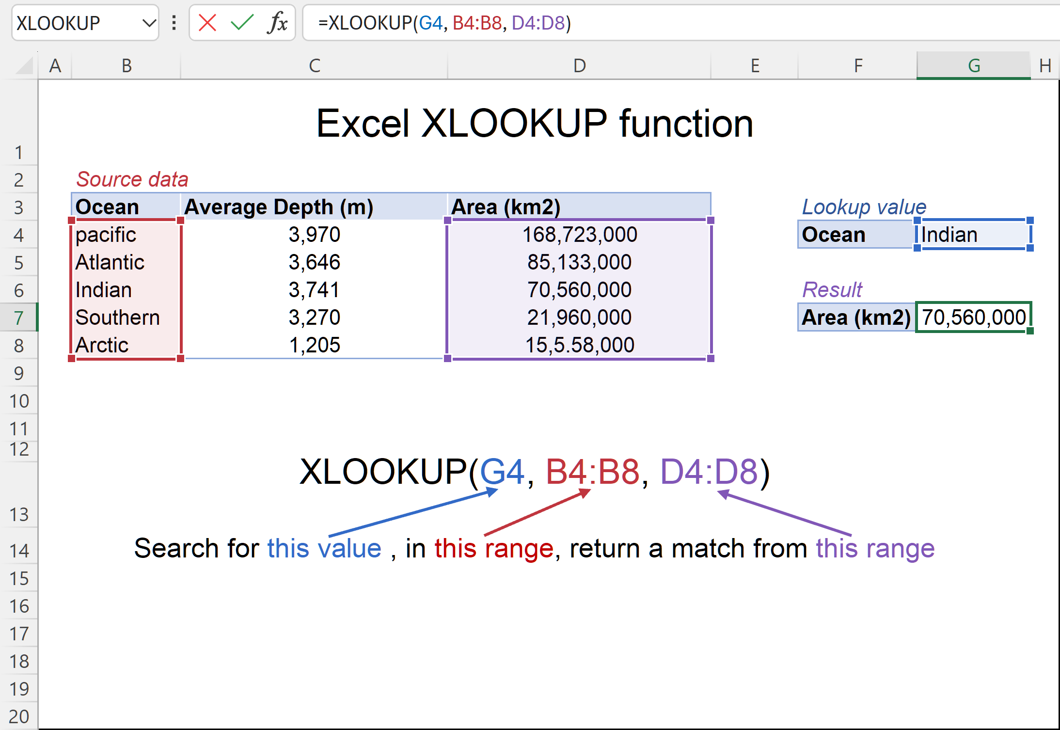
XLOOKUP Formula in Excel with Example
To better understand how XLOOKUP works, let’s explore an example:
Imagine you have a list of employee names and their respective salaries, and you want to look up the salary of a specific employee.
Employee Name
Salary
John
50,000
Mary
60,000
Steve
55,000
Emma
65,000
In this case, to look up the salary of “Steve”, you would use the following formula:
less
=XLOOKUP("Steve", A2:A5, B2:B5)
Here, “Steve” is the lookup_value, A2:A5 is the lookup_array containing the employee names, and B2:B5 is the return_array containing the salaries. The result would be 55,000, the salary of Steve.
XLOOKUP vs VLOOKUP
The introduction of XLOOKUP led to the gradual obsolescence of the older lookup functions like VLOOKUP. While both functions can retrieve values from a table or range, there are several key differences between XLOOKUP and VLOOKUP.
Flexibility in Lookup Direction:
VLOOKUP can only search for the lookup value in the first column of a table and return a corresponding value from columns to the right.
XLOOKUP, on the other hand, can search in any column or row and return values from any other column or row, not necessarily to the right. This makes XLOOKUP much more versatile.
Handling Missing Values:
VLOOKUP returns an error (typically #N/A) if the lookup value is not found.
XLOOKUP allows you to define a custom value to return when the lookup value is not found, such as “Not Found” or any other text or value.
Performance:
VLOOKUP requires you to specify the column number for the result, which can be cumbersome if the table structure changes (i.e., if columns are rearranged).
XLOOKUP eliminates the need to reference column numbers, as it directly refers to the column from which to retrieve the result.
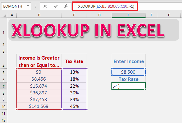
Approximate Match:
VLOOKUP defaults to an approximate match unless specified as an exact match using the fourth argument.
XLOOKUP defaults to an exact match but can be configured to perform an approximate match as well.
XLOOKUP Not Available in Excel
Despite being available in Excel 365 and Excel 2021, some older versions of Excel (Excel 2019 and earlier) do not have access to the XLOOKUP function. If you are working with a version of Excel that does not support XLOOKUP, you can use alternatives such as VLOOKUP or INDEX-MATCH, which can mimic some of the functionalities of XLOOKUP, though with more complexity.
To check whether XLOOKUP is available in your version of Excel, you can simply try typing the function in a cell. If Excel recognizes it, then you have access to it. If it does not, you will need to upgrade to a version that supports XLOOKUP.
How to Use XLOOKUP in Excel with Two Sheets
XLOOKUP is highly effective when you need to retrieve data from multiple sheets. Suppose you have two sheets: “Sheet1” and “Sheet2”. Sheet1 contains employee names, and Sheet2 contains their salaries.
Sheet1:
Employee Name
John
Mary
Steve
Emma
Sheet2:
Employee Name
Salary
John
50,000
Mary
60,000
Steve
55,000
Emma
65,000
To find the salary of “Steve” from Sheet2 while working in Sheet1, use the following formula:
less
=XLOOKUP(A2, Sheet2!A2:A5, Sheet2!B2:B5)
In this formula:
A2 is the lookup value from Sheet1 (the employee name).
Sheet2!A2:A5 is the lookup range from Sheet2 (employee names).
Sheet2!B2:B5 is the return range from Sheet2 (salaries).
XLOOKUP Exact Match
When using XLOOKUP, you can specify that you want an exact match. By default, XLOOKUP performs an exact match search, but you can explicitly indicate it by setting the match_mode argument to 0.
For example, to search for an exact match of “John” in a list of names, use the following formula:
less
=XLOOKUP("John", A2:A5, B2:B5, "Not Found", 0)
This will search for “John” and return the corresponding value from column B (salary). If “John” is not found, the function will return “Not Found”.
XLOOKUP Return Array
One of the powerful features of XLOOKUP is the ability to return an array of values rather than a single result. This allows you to perform advanced lookups without needing additional functions.
For example, if you wanted to return a list of salaries for a range of employees, you can use the XLOOKUP function to retrieve multiple matching values. However, note that this functionality is more commonly used in the context of dynamic arrays, which is supported in Excel 365 and Excel 2021.
XLOOKUP Not Working
If XLOOKUP is not working, there could be several reasons behind the issue:
Version Incompatibility: As mentioned earlier, if you’re using a version of Excel older than Excel 365 or Excel 2021, XLOOKUP will not be available.
Incorrect Syntax: Double-check your function’s syntax and ensure all arguments are correct.
Array Mismatch: Ensure that the lookup_array and return_array are of the same size and shape.
Data Formatting: Ensure that the data you’re searching through is formatted consistently (e.g., no leading or trailing spaces, correct data types).
Circular References: Avoid circular references in your formulas, as these can prevent XLOOKUP from working properly.
Conclusion
The XLOOKUP function in Excel is a game-changer for those looking to simplify and streamline their data lookups. With its improved flexibility, ease of use, and ability to handle more complex lookup scenarios, XLOOKUP offers significant advantages over older functions like VLOOKUP and HLOOKUP. Whether you’re working across multiple sheets, performing exact matches, or returning entire arrays, XLOOKUP provides the tools to work more efficiently and effectively with your data.
Needs help with similar assignment?
We are available 24x7 to deliver the best services and assignment ready within 3-4 hours? Order a custom-written, plagiarism-free paper
https://getspsshelp.com/wp-content/uploads/2024/12/logo-8.webp00Besttutorhttps://getspsshelp.com/wp-content/uploads/2024/12/logo-8.webpBesttutor2025-01-31 08:30:082025-05-31 10:28:17XLOOKUP Function in Excel: A Comprehensive Guide|2025
The FILTER Function in Excel: Learn how to filter and extract data dynamically for efficient analysis. Master this powerful tool to streamline workflows and enhance productivity!
Excel has long been regarded as one of the most powerful tools for data manipulation and analysis. Its functionalities have evolved over the years to provide users with more efficient ways to handle large datasets. One of the most powerful features in Excel for filtering data is the FILTER function. This function allows users to return a specific subset of data that meets defined criteria. However, the availability and usage of the FILTER function depend on the version of Excel you are using. This paper explores the functionality of the FILTER function in different versions of Excel, its uses with multiple criteria, and how it can be applied to both single and multiple columns of data.
Overview of the FILTER Function in Excel
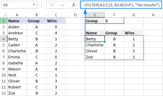
The FILTER function is a dynamic array function introduced in Excel 365 and Excel 2021. It allows users to filter a range of data based on criteria they specify, with the result being a dynamic array that automatically updates when the source data changes. The basic syntax of the function is:
css
=FILTER(array, include, [if_empty])
Where:
array refers to the range or array of data that you want to filter.
include is a Boolean array or expression that defines the filtering conditions.
[if_empty] is an optional argument that specifies the value to return if no data meets the criteria.
This function can save time for Excel users who need to extract subsets of data based on specific conditions.
Availability of the FILTER Function
The FILTER function is not available in all versions of Excel. Users of Excel versions prior to Excel 365 or Excel 2021 do not have access to this function. Therefore, users working with older versions of Excel, such as Excel 2016 or Excel 2019, will need to use alternative methods, such as traditional filter tools or advanced formulas (like IF, INDEX, or MATCH) to achieve similar results.
In Excel 2016, the FILTER function is not available. Users of this version will have to rely on manual filtering or create complex formulas to simulate filtering results.
In Excel 2019, the FILTER function was not initially available at its release but was later included in the update for users with Microsoft 365 subscriptions. However, users who do not have access to the dynamic array functions in Excel 2019 will not be able to use the FILTER function and will need to explore alternative methods.
Excel FILTER Function with Multiple Criteria
One of the powerful features of the FILTER function is its ability to apply multiple criteria. When filtering data based on more than one condition, users can combine multiple logical expressions using the * (AND) or + (OR) operators. The result is a filtered array that meets all the conditions specified.
Example: Excel FILTER Function with Multiple Criteria (AND condition)
Suppose you have a dataset of sales data with columns for Salesperson, Product, and Amount. If you want to filter the data to show sales made by a specific salesperson for a particular product, you can use the FILTER function with multiple criteria combined with the * operator, which functions like an AND condition.
The A2:A10="John" condition checks for records where the salesperson is “John.”
The B2:B10="Laptop" condition filters for rows where the product is a “Laptop.”
The * operator ensures that both conditions must be true for the data to be included in the result.
Example: Excel FILTER Function with Multiple Criteria (OR condition)
Alternatively, if you want to filter the data to show sales by “John” or “Jane,” you can use the + operator, which functions like an OR condition.
less
=FILTER(A2:C10, (A2:A10="John")+(A2:A10="Jane"))
This formula will return all records where the salesperson is either “John” or “Jane.”
Excel FILTER Function with Multiple Columns
The FILTER function in Excel is not limited to filtering data in a single column. It can also be applied to filter data across multiple columns. By providing a multi-column range as the array argument, users can filter based on multiple columns of data simultaneously.
Example: Filtering Data Across Multiple Columns
Imagine you have a dataset that includes sales information, including salesperson, product, and amount. You can filter the data by applying conditions to multiple columns at once.
ruby
=FILTER(A2:C10, (A2:A10="John")*(C2:C10>5000))
In this example:
The A2:A10="John" condition filters for sales made by “John.”
The C2:C10>5000 condition filters for sales amounts greater than 5000.
The * operator ensures that both conditions must be met.
This formula will return the sales data for “John” with amounts greater than 5000.
Excel FILTER Function for Multiple Values
The FILTER function can also handle multiple values in a single column, allowing users to filter data based on a list of values. This can be done by using the ISNUMBER and MATCH functions inside the FILTER function.
Example: Filtering Multiple Values from a Single Column
Suppose you want to filter data for multiple products, such as “Laptop,” “Phone,” and “Tablet.” You can use the following formula:
The MATCH function checks if the value in the B2:B10 range matches any of the values in the list {"Laptop", "Phone", "Tablet"}.
The ISNUMBER function returns TRUE if a match is found, allowing the FILTER function to include those rows in the result.
This formula filters the dataset to include only the rows where the product is one of the specified values.
Excel FILTER Function in Excel 2019
In Excel 2019, the FILTER function is not available as a standard feature for all users. However, users with access to Office 365 or those who have updated their Excel 2019 with Microsoft 365 subscription may be able to use the FILTER function. For those without access, alternatives like array formulas or advanced filtering features like AutoFilter or the Advanced Filter tool can be used to filter data based on specific criteria.
In Excel 2019, users often rely on the Advanced Filter tool, which allows for filtering based on complex criteria. To use the Advanced Filter, users need to define a criteria range and then apply the filter to the data. This process is more manual than the FILTER function but still provides powerful filtering capabilities.
Excel FILTER Function for Multiple Criteria in the Same Column
The FILTER function can also be used to filter data based on multiple criteria within the same column. For instance, if you want to filter a list of sales data where the salesperson is either “John” or “Jane,” you can use the following formula:
less
=FILTER(A2:C10, (A2:A10="John")+(A2:A10="Jane"))
This formula returns all rows where the salesperson is either “John” or “Jane.” The + operator ensures that any record with either of the names will be included in the result.
Conclusion
The FILTER function is a powerful tool in Excel that simplifies the process of extracting specific subsets of data based on criteria. For users with Excel 365 or Excel 2021, the FILTER function offers a simple, flexible way to filter data across multiple criteria, columns, and values. However, for users of older versions of Excel, like Excel 2016 or Excel 2019, alternative methods, such as Advanced Filters and complex formulas, may be required. Understanding how to use the FILTER function effectively can significantly enhance productivity and streamline data analysis tasks in Excel.
GetSPSSHelp is the best choice for mastering the FILTER function in Excel because of our expert guidance and student-focused approach. Our team simplifies complex concepts, providing clear, step-by-step instructions to help you filter and extract data effortlessly. We ensure accuracy, save time, and enhance your understanding of Excel. With affordable pricing, 24/7 support, and a commitment to quality, we make learning FILTER stress-free and effective. Whether you’re a beginner or advanced user, GetSPSSHelp empowers you to excel in data analysis. Trust us for reliable, professional assistance that boosts your skills and confidence!
Needs help with similar assignment?
We are available 24x7 to deliver the best services and assignment ready within 3-4 hours? Order a custom-written, plagiarism-free paper
https://getspsshelp.com/wp-content/uploads/2024/12/logo-8.webp00Besttutorhttps://getspsshelp.com/wp-content/uploads/2024/12/logo-8.webpBesttutor2025-01-31 08:28:032025-04-08 20:51:42The FILTER Function in Excel: An In-Depth Guide|2025
The UNIQUE Function in Excel: Learn how to extract unique values from datasets for efficient data analysis. Master this powerful tool to streamline workflows and enhance productivity!
Excel, one of the most widely used spreadsheet applications, continues to evolve with each version, providing users with a range of tools that streamline data analysis, manipulation, and presentation. One of the more recent additions to Excel is the UNIQUE function, which allows users to easily extract distinct values from a list of data.
While this function is highly useful for simplifying workflows, it’s important to understand its availability, usage, and alternatives, especially for users on older versions of Excel. In this paper, we will discuss the UNIQUE function in detail, focusing on its role in Excel 2019 and later versions, its availability in Excel 2016, alternatives for older versions, its application in multiple criteria, and its integration with Excel VBA.
Understanding the UNIQUE Function
The UNIQUE function in Excel enables users to filter out duplicate values from a range or array, leaving only distinct values behind. The syntax for this function is simple:
css
=UNIQUE(array, [by_col], [exactly_once])
array: The range or array from which you want to extract unique values.
by_col (optional): A logical value (TRUE or FALSE) that specifies whether to compare values by rows or columns. By default, Excel compares values by rows (FALSE).
exactly_once (optional): If TRUE, the function will return only values that appear exactly once in the array.
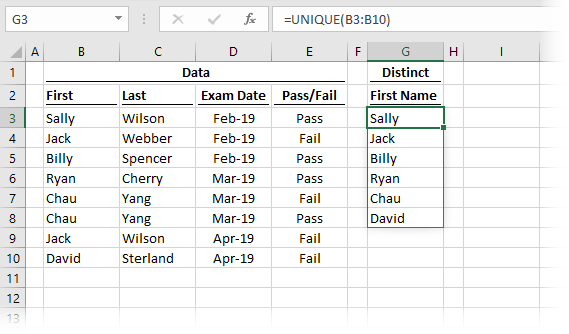
For example, if you have a list of names in a column and want to extract the unique names, you would use the formula:
scss
=UNIQUE(A1:A10)
This would return only the unique names from the specified range.
Unique Formula in Excel 2016
Despite being a powerful tool for data analysis, the UNIQUE function is not available in Excel 2016. In this version, users must rely on alternative methods to extract unique values. While this limitation can be frustrating, Excel 2016 still offers several options to simulate the functionality of the UNIQUE function.
One common method is to use a combination of other Excel functions, such as IF, COUNTIF, or SUMPRODUCT. For instance, to extract unique values from a list in Excel 2016, users can use an array formula with COUNTIF to identify the first occurrence of each item.
Example:
swift
=IF(COUNTIF($A$1:$A$10, A1) =1, A1, "")
This formula checks if the value in cell A1 appears only once in the range A1:A10. If it does, it returns the value; otherwise, it returns an empty string.
However, these workarounds can be cumbersome and are not as efficient as the built-in UNIQUE function in later versions.
Unique Function in Excel Shortcut
While the UNIQUE function itself does not have a dedicated keyboard shortcut in Excel, you can still use Excel’s powerful keyboard shortcuts to navigate and apply the function quickly.
For instance, if you have a range of data and want to extract unique values, the process would generally involve the following steps:
Select the cell where you want to enter the formula.
Type =UNIQUE(, then select the range of data.
Press Enter.
To enhance efficiency, you can use AutoFill to quickly copy the formula to adjacent cells after entering it in the first cell. This process can be sped up by utilizing the Ctrl + Shift + Arrow keys to select large ranges.
Additionally, if you are working with Excel’s more complex formulas, you can press Alt + E + S to access the Paste Special menu, which can help you apply the UNIQUE function to a range more effectively, especially if you need to transpose the data or remove duplicates.
Alternatives to the UNIQUE Function in Excel
For users who are working in versions of Excel that do not support the UNIQUE function (such as Excel 2016), there are several alternative methods for extracting unique values:
Using PivotTables
One of the most efficient ways to extract unique values in Excel 2016 is by using a PivotTable. A PivotTable allows users to summarize data and display unique values without the need for complex formulas.
Select the range of data.
Go to the Insert tab and select PivotTable.
In the PivotTable Field List, drag the desired field to the Rows area.
This will display the unique values from the selected field.
Removing Duplicates
Another simple method is using Excel’s built-in Remove Duplicates feature:
Select the data range.
Go to the Data tab.
Click Remove Duplicates in the Data Tools group.
In the dialog box, choose the columns from which you want to remove duplicates.
This method is useful for cleaning data, but it alters the original data range and does not provide dynamic updates like the UNIQUE function.
Using Advanced Filter
Excel also provides the Advanced Filter option to extract unique values:
Select the range of data.
Go to the Data tab and click on Advanced in the Sort & Filter group.
Choose the option Copy to another location.
Check the box Unique records only and specify the destination.
This method allows users to copy the unique values to a new location without affecting the original data set.
UNIQUE Function in Excel 2019
The UNIQUE function is available in Excel 2019 and later versions, including Excel for Microsoft 365. Excel 2019 users can now take full advantage of this function to extract distinct values from their data with ease.
One notable feature of the UNIQUE function in Excel 2019 is its dynamic array behavior, which means that it automatically spills the results into adjacent cells when you press Enter. This eliminates the need for additional formulas or copying and pasting values.
For example, if you have a list of numbers in A1:A10 and want to find the unique values, you can simply enter:
scss
=UNIQUE(A1:A10)
The function will automatically expand to display the unique values in the cells below.
How to Use the UNIQUE Function in Excel
Using the UNIQUE function is straightforward, but there are a few variations that can be useful in more complex scenarios.
Basic Example
To extract unique values from a list, use:
scss
=UNIQUE(A1:A10)
This will return all unique values from the range A1:A10.
Unique Values Based on Multiple Criteria
You can use the UNIQUE function with multiple criteria by combining it with other functions such as FILTER. For example, if you want to extract unique values from a list based on a specific condition, you could use:
less
=UNIQUE(FILTER(A1:B10, B1:B10="Condition"))
This formula returns unique values from column A where the corresponding value in column B meets the specified condition.
Exact Matches
If you want the UNIQUE function to return only values that appear exactly once, use the exactly_once argument:
php
=UNIQUE(A1:A10, , TRUE)
This will return only the values in A1:A10 that appear exactly once in the range.
Unique Function in Excel VBA
In addition to using the UNIQUE function in Excel formulas, you can also integrate it into Excel VBA (Visual Basic for Applications) to automate tasks. To use the UNIQUE function in VBA, you can employ the WorksheetFunction object.
Example VBA code to use the UNIQUE function:
vba
Sub ExtractUniqueValues()

Dim rng As Range

Dim uniqueValues As Variant
‘ Define the range
Set rng = Range(“A1:A10”)‘ Get unique values using the UNIQUE function
uniqueValues = Application.WorksheetFunction.Unique(rng)‘ Output unique values to another range
Range(“B1”).Resize(UBound(uniqueValues), 1).Value = Application.Transpose(uniqueValues)
End Sub
This code extracts the unique values from the range A1:A10 and outputs them in column B. By using VBA, you can automate tasks that involve extracting unique values across multiple sheets or large data sets.
Conclusion
The UNIQUE function in Excel is a powerful tool for simplifying data analysis by extracting distinct values from a list or array. While not available in Excel 2016, users can still rely on alternative methods such as PivotTables, advanced filtering, or removing duplicates. Excel 2019 and later versions offer full support for the UNIQUE function, making it easier for users to work with dynamic arrays and handle more complex data analysis tasks. Additionally, the function can be used in combination with other Excel features like multiple criteria and VBA to enhance its versatility and automation capabilities. As Excel continues to evolve, functions like UNIQUE provide users with more powerful tools to streamline their data workflows.
GetSPSSHelp is the best choice for mastering the UNIQUE function in Excel because of our expert guidance and student-focused approach. Our team simplifies complex concepts, providing clear, step-by-step instructions to help you extract unique values effortlessly. We ensure accuracy, save time, and enhance your understanding of Excel. With affordable pricing, 24/7 support, and a commitment to quality, we make learning the UNIQUE function stress-free and effective. Whether you’re a beginner or advanced user, GetSPSSHelp empowers you to excel in data analysis. Trust us for reliable, professional assistance that boosts your skills and confidence!
Needs help with similar assignment?
We are available 24x7 to deliver the best services and assignment ready within 3-4 hours? Order a custom-written, plagiarism-free paper
https://getspsshelp.com/wp-content/uploads/2024/12/logo-8.webp00Besttutorhttps://getspsshelp.com/wp-content/uploads/2024/12/logo-8.webpBesttutor2025-01-31 08:26:342025-09-08 11:10:13The UNIQUE Function in Excel: A Comprehensive Overview|2025
The TRANSPOSE Function in Excel: Learn how to switch rows and columns for efficient data organization. Master this powerful tool to streamline workflows and enhance productivity!
Excel is a powerful tool used for managing, analyzing, and visualizing data. One of the many features that can greatly enhance productivity is the TRANSPOSE function. This function enables users to switch data from rows to columns or vice versa, offering flexibility in organizing and presenting information. In this paper, we will explore the various aspects of the TRANSPOSE function in Excel, including its use, formulas, shortcuts, and troubleshooting tips. Additionally, we will cover specific scenarios, such as dynamic transposing, transposing based on criteria, and more.
Introduction to the TRANSPOSE Function
The TRANSPOSE function in Excel allows users to swap rows and columns in a data set. This is particularly useful when the arrangement of data needs to be restructured for analysis, reporting, or presentation. Whether you want to turn a horizontal list into a vertical one, or vice versa, the TRANSPOSE function can help.
At its core, the function takes a range of cells (either a row or a column) and rearranges it into the opposite direction, without altering the original data. The general syntax for the TRANSPOSE function is as follows:
excel
=TRANSPOSE(array)
Where array is the range of cells you want to transpose.
Transpose Row to Column in Excel
One of the most common uses of the TRANSPOSE function is to transpose row to column in Excel. This is particularly useful when you have data arranged horizontally, such as a list of months or a sequence of numerical values, and you need to convert it into a vertical format. For instance, if you have the following data in a row:
| January | February | March |
You can use the TRANSPOSE function to convert it into a column format, like this:
| January | | February | | March |
To do this, follow these steps:
Select the range where you want the transposed data to appear.
Enter the formula =TRANSPOSE(A1:C1), where A1:C1 is the range of cells you want to transpose.
Press Ctrl + Shift + Enter (for array formulas) to complete the process.
The data will now appear in a column instead of a row.
Transpose Shortcut in Excel
For users who prefer quick and efficient ways to work within Excel, the transpose shortcut in Excel can be a time-saver. Instead of entering a formula, you can use the following steps to transpose data with a keyboard shortcut:
Copy the data you wish to transpose (use Ctrl + C).
Select the destination range where you want to paste the transposed data.
Right-click the first cell in the destination range.
Under the Paste Special menu, click Transpose. Alternatively, you can press Alt + E + S + E, followed by Enter.
This method allows you to quickly transpose data without the need for writing a formula.
Excel TRANSPOSE Formula Columns to Rows
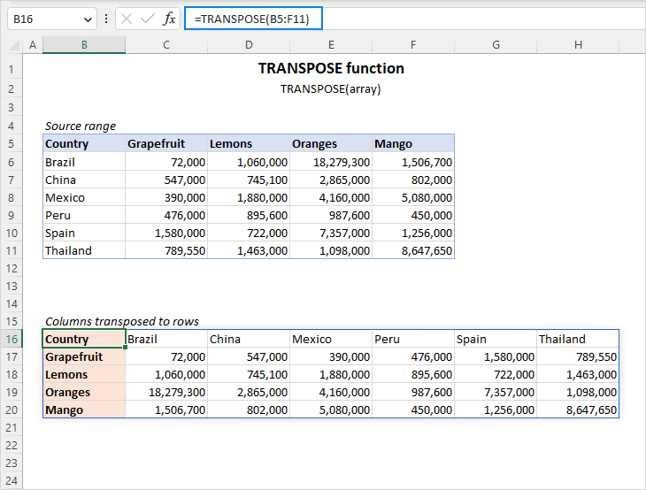
In some cases, you might need to transpose columns to rows in Excel. This scenario is the inverse of the previous one. If you have a list of vertical data in a column and want to convert it into a horizontal row, the TRANSPOSE function works just as well.
For example, suppose you have the following data in a column:
| 1 | | 2 | | 3 |
To transpose this data into a row, follow these steps:
Select the destination range where you want to transpose the data.
Enter the formula =TRANSPOSE(A1:A3), where A1:A3 represents the range of cells you want to transpose.
Press Ctrl + Shift + Enter (for array formulas).
The data will now appear in a row format:
| 1 | 2 | 3 |
Troubleshooting: Excel TRANSPOSE Function Not Working
While the TRANSPOSE function is generally reliable, there are times when it may not work as expected. Here are a few common reasons for issues:
Array Formula Errors: The TRANSPOSE function requires array formulas in some cases. If you’re not using Ctrl + Shift + Enter when inputting the formula, Excel may not recognize it as an array formula. To fix this, ensure you are pressing Ctrl + Shift + Enter when entering the formula.
Mismatched Range Sizes: The range you’re transposing must have the correct number of rows and columns to fit the new layout. For example, if you are transposing a 3×1 range into a row, the destination should be a 1×3 range. If the sizes do not match, Excel will return an error.
Merged Cells: The presence of merged cells in the source data may prevent the TRANSPOSE function from working correctly. To resolve this, unmerge the cells in the source range before transposing.
Too Large a Range: If the range of cells you’re trying to transpose is too large, it can result in an error or cause Excel to become unresponsive. If this occurs, try breaking the range into smaller sections.
Non-Numeric Data: The TRANSPOSE function works with both numeric and non-numeric data, but if there is an issue with a specific type of data (e.g., formulas that reference external workbooks), the function may fail.
How to Convert Vertical to Horizontal in Excel Using Formula
Converting data from vertical to horizontal (or vice versa) can be achieved using the TRANSPOSE function. For example, if you have data arranged in a column and you want to convert it into a row, simply use the following steps:
Copy the vertical data range (for example, A1:A5).
Select the range where you want the horizontal data to appear.
Enter the formula =TRANSPOSE(A1:A5).
Press Ctrl + Shift + Enter.
This method works when you need to convert data from a vertical list to a horizontal one.
Excel Transpose Multiple Rows in Group to Columns
The Excel transpose multiple rows in group to columns feature is helpful when you need to transpose data in a more complex scenario, such as when you want to group several rows and transpose them into multiple columns.
For instance, suppose you have the following data:
Name
Age
City
John
25
NY
Sara
30
LA
Mike
35
SF
You can use the TRANSPOSE function to rearrange this data into a set of columns. Here’s how you would do it:
Select the destination where you want the transposed data.
Enter the formula =TRANSPOSE(A1:C3).
Press Ctrl + Shift + Enter.
The result would look something like this:
Name
John
Sara
Mike
Age
25
30
35
City
NY
LA
SF
This method works well when you need to transpose data with multiple rows and group them into columns.
Dynamic Transpose in Excel
The dynamic transpose in Excel allows you to transpose data that updates automatically when the source data changes. This is a great feature when you want the transposed data to reflect any changes in real-time without having to re-enter the formula.
To set up dynamic transposing, use the TRANSPOSE function in combination with dynamic ranges. For instance, you can use the OFFSET function to create a dynamic range, and then transpose that range. The formula would look something like this:
excel
=TRANSPOSE(OFFSET(A1,0,0,COUNTA(A:A),1))
This formula creates a dynamic range starting from A1 and dynamically adjusts based on the number of rows in column A. The COUNTA(A:A) function counts the non-empty cells in the range and adjusts the number of rows accordingly.
Excel Transpose Rows to Columns Based on Criteria
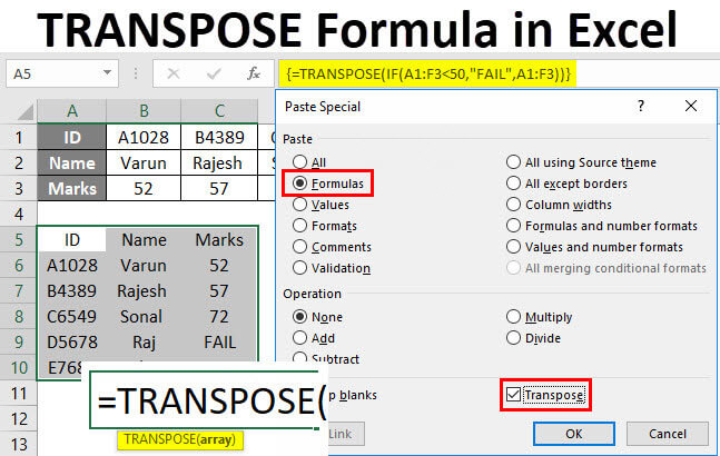
You can also use the TRANSPOSE function in Excel to transpose rows to columns based on specific criteria. This can be done using IF statements in combination with the TRANSPOSE function. For example, if you have data where certain rows meet specific criteria, and you only want to transpose those rows that meet the condition, you can use an array formula.
For instance, you can use the following formula to transpose data in rows where the value in column A is greater than 10:
excel
=TRANSPOSE(IF(A1:A5>10,B1:B5,""))
This formula will transpose only the values in column B where the corresponding values in column A are greater than 10.
Conclusion
The TRANSPOSE function in Excel is a powerful tool that allows users to manipulate data by changing the orientation of rows and columns. Whether you are looking to convert a row to a column, transpose based on specific criteria, or use shortcuts for quick transposing, the TRANSPOSE function offers flexibility and ease. However, users should be aware of common issues such as array formula errors, merged cells, and large ranges, which can prevent the function from working correctly. By understanding the function’s syntax and how it can be applied in various scenarios, users can make the most of Excel’s capabilities for data manipulation.
GetSPSSHelp is the best choice for mastering the TRANSPOSE function in Excel because of our expert guidance and student-focused approach. Our team simplifies complex concepts, providing clear, step-by-step instructions to help you switch rows and columns effortlessly. We ensure accuracy, save time, and enhance your understanding of Excel. With affordable pricing, 24/7 support, and a commitment to quality, we make learning the TRANSPOSE function stress-free and effective. Whether you’re a beginner or advanced user, GetSPSSHelp empowers you to excel in data analysis. Trust us for reliable, professional assistance that boosts your skills and confidence!
Needs help with similar assignment?
We are available 24x7 to deliver the best services and assignment ready within 3-4 hours? Order a custom-written, plagiarism-free paper
https://getspsshelp.com/wp-content/uploads/2024/12/logo-8.webp00Besttutorhttps://getspsshelp.com/wp-content/uploads/2024/12/logo-8.webpBesttutor2025-01-31 08:24:582025-02-01 12:10:28The TRANSPOSE Function in Excel: A Comprehensive Overview|2025
ISERROR and IFERROR Functions in Excel: Learn how to handle errors in formulas for efficient data analysis. Master these essential tools to streamline workflows and enhance productivity!
Microsoft Excel has become a powerful tool for both professionals and casual users for performing a variety of calculations, organizing data, and handling errors. Among the various functions available, two frequently used functions are ISERROR and IFERROR. These functions are used to identify and handle errors that can occur in Excel formulas, helping users to create cleaner, more readable spreadsheets.
In this paper, we will explore the ISERROR and IFERROR functions in detail, comparing their features, applications, and differences. We will also look at how they can be used together with functions like VLOOKUP and how these error-handling tools are applied in Excel 365. Additionally, the use of multiple conditions with these functions and how to return blanks for errors will also be examined.
ISERROR Function in Excel
The ISERROR function in Excel is used to check whether a given expression or formula results in an error. If the formula results in an error, the ISERROR function returns TRUE, and if there is no error, it returns FALSE. The primary use of ISERROR is to trap errors within formulas and take corrective actions based on whether an error occurs or not.
Syntax of ISERROR:
excel
=ISERROR(value)
value: This is the expression or formula to evaluate. If the formula evaluates to any type of error, ISERROR returns TRUE. Otherwise, it returns FALSE.
Example of ISERROR:
Suppose you have a formula in cell A1 that divides the value in B1 by the value in C1. If C1 is zero, Excel will return an error. You can wrap the division formula with ISERROR to check for errors:
excel
=ISERROR(A1/B1)
If C1 is zero, the formula will return TRUE indicating that there is an error.
ISERROR Function in Excel with VLOOKUP
The VLOOKUP function is one of Excel’s most commonly used lookup functions. However, when VLOOKUP cannot find a matching value, it returns an #N/A error. Using ISERROR with VLOOKUP can help in managing these errors effectively.
Example of ISERROR with VLOOKUP:
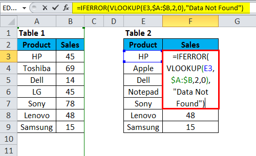
Consider you are using VLOOKUP to search for a value in column A and return a corresponding value from column B. If the lookup value is not found, VLOOKUP will return #N/A. You can use ISERROR to return a custom message or value instead of the error.
If VLOOKUP cannot find the value in D1, ISERROR returns TRUE, and the message “Not Found” is displayed.
If VLOOKUP is successful, it returns the corresponding value from column B.
Limitations of ISERROR
While the ISERROR function is quite useful, it has its limitations. One of the key drawbacks is that it catches all errors, including #VALUE!, #REF!, and #DIV/0!, without distinguishing between them. Therefore, it may not be suitable for situations where you want to handle different types of errors separately.
IFERROR Function in Excel
The IFERROR function was introduced to provide a more flexible and straightforward way to handle errors compared to ISERROR. The IFERROR function not only checks for errors but also allows you to specify a value to return when an error occurs.
Syntax of IFERROR:
excel
=IFERROR(value, value_if_error)
value: This is the expression or formula to evaluate.
value_if_error: This is the value to return if an error is found in the expression.
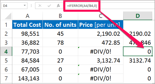
Example of IFERROR:
If you want to divide A1 by B1, and return “Error” when B1 is zero, you can use IFERROR as follows:
excel
=IFERROR(A1/B1, "Error")
In this case:
If the division does not result in an error, the result will be displayed.
If there is an error (e.g., B1 is zero), the result will be “Error”.
ISERROR vs IFERROR
While both ISERROR and IFERROR serve the same general purpose of handling errors, they are different in terms of their syntax and functionality.
Key Differences:
Functionality:
ISERROR only returns TRUE or FALSE based on whether an error occurs.
IFERROR allows you to define a custom response if an error occurs, providing more control over the outcome.
Syntax:
ISERROR requires an additional formula to process the error, such as using it within an IF statement.
IFERROR allows you to handle errors directly within the function, without needing to wrap it in a separate IF statement.
Error Handling:
ISERROR can only flag errors without correcting them or offering an alternative value.
IFERROR can directly return an alternative value when an error occurs, making it more user-friendly.
Example of ISERROR vs IFERROR:
To check if A1/B1 results in an error and return “Error” if it does, using ISERROR:
excel
=IF(ISERROR(A1/B1), "Error", A1/B1)
Using IFERROR:
excel
=IFERROR(A1/B1, "Error")
In this case, both formulas yield the same result, but IFERROR is much simpler and easier to use.
ISERROR and IFERROR Functions in Excel 365
In Excel 365, both ISERROR and IFERROR functions are available, but there are additional functions that offer more specialized error-handling capabilities. One of these is the IFNA function, which handles #N/A errors specifically. However, IFERROR and ISERROR still remain highly relevant.
Excel 365 also includes additional dynamic array features and the LET function, which can make error-handling more efficient when combined with ISERROR and IFERROR.
Example in Excel 365:
Suppose you want to check if A1 is greater than B1, and if either cell contains an error, return “Check Values”:
This formula works seamlessly in Excel 365, and the IFERROR function handles any errors in the comparison.
Excel IF(ISERROR) Multiple Conditions
The IF(ISERROR(…)) combination can also be used with multiple conditions, allowing you to check for errors under specific circumstances and apply different responses accordingly.
Example of Multiple Conditions:
If you have A1/B1 and want to check if the result is an error, but only when B1 is not empty, you can use:
excel
=IF(B1<>"", IF(ISERROR(A1/B1), "Error", A1/B1), "B1 is empty")
Here, the formula first checks if B1 is empty. If not, it performs the division and checks for errors.
Excel IF Error Then Blank
In many cases, you may want to return a blank cell instead of a custom error message when an error occurs. This can be achieved by simply leaving the value_if_error argument blank in the IFERROR function.
Example of Returning Blank on Error:
excel
=IFERROR(A1/B1, "")
In this case, if A1/B1 results in an error, the formula returns a blank cell instead of an error message.
Conclusion
The ISERROR and IFERROR functions in Excel are invaluable tools for error handling, each serving distinct purposes based on the user’s needs. While ISERROR is useful for identifying errors and flagging them, IFERROR offers more flexibility by allowing the user to specify alternative values when an error occurs. In Excel 365, these functions continue to play a vital role in error management, and their use in conjunction with other functions like VLOOKUP and IF makes Excel more powerful and efficient.
Whether you’re handling simple division errors, complex lookups, or managing multiple conditions, understanding the differences between ISERROR and IFERROR, and knowing how to apply them, is essential for creating robust and error-free spreadsheets.
Needs help with similar assignment?
We are available 24x7 to deliver the best services and assignment ready within 3-4 hours? Order a custom-written, plagiarism-free paper
https://getspsshelp.com/wp-content/uploads/2024/12/logo-8.webp00Besttutorhttps://getspsshelp.com/wp-content/uploads/2024/12/logo-8.webpBesttutor2025-01-31 08:23:302025-05-31 10:27:58ISERROR and IFERROR Functions in Excel|2025
Understanding the AND, OR, and NOT Functions in Excel: Learn how to perform logical operations and streamline your data analysis. Master these essential tools for efficient workflows and reporting!
Microsoft Excel is an essential tool for data analysis, calculations, and decision-making. Among its many powerful features, logical functions are pivotal for evaluating conditions and making decisions based on specific criteria. Logical functions in Excel include AND, OR, and NOT, which allow users to test multiple conditions and return either TRUE or FALSE. These functions are essential in filtering data, performing conditional calculations, and building more complex formulas. This paper will explore the workings of the AND, OR, and NOT functions in Excel, provide multiple examples, and demonstrate their applications with multiple criteria.
What Are Logical Functions in Excel?
Logical functions are built to evaluate whether certain conditions are met. These functions help in performing decision-making tasks, like checking if specific criteria are true or false. In Excel, logical functions include:
AND
OR
NOT
IF
IFERROR
IFNA
XOR
IFIFS
SWITCH
CHOOSE
For this paper, we will focus on the three fundamental logical functions: AND, OR, and NOT.
The AND Function in Excel
The AND function is used to test multiple conditions simultaneously. It returns TRUE only when all specified conditions are true. If any of the conditions are false, the function returns FALSE.
condition1, condition2, …, conditionN are the logical conditions or expressions to evaluate.
Example of AND Function in Excel
Imagine a scenario where a company wants to determine whether an employee qualifies for a bonus based on two conditions:
The employee must have worked for more than 5 years.
The employee must have a performance rating above 8.
Here’s how the formula can be structured:
excel
=AND(A2>5, B2>8)
In this example:
A2 refers to the number of years the employee has worked.
B2 refers to the performance rating of the employee.
If both conditions are true (the employee has worked for more than 5 years and has a performance rating above 8), the formula returns TRUE; otherwise, it returns FALSE.
AND Function with Multiple Criteria
The AND function can also handle more than two conditions. For instance, if an employee must meet three conditions to qualify for a bonus:
Worked for more than 5 years
Performance rating above 8
Completed a certain project
The formula becomes:
excel
=AND(A2>5, B2>8, C2="Completed")
This formula will return TRUE if the employee satisfies all three conditions.
The OR Function in Excel
The OR function is another logical function that tests multiple conditions, but it returns TRUE if any of the conditions are true. It only returns FALSE if all conditions are false.
Syntax of the OR Function
excel
=OR(condition1, condition2, ..., conditionN)
Where:
condition1, condition2, …, conditionN are the logical conditions or expressions to evaluate.
Example of OR Function in Excel
Let’s say a student is eligible for a scholarship if they meet one of the following two conditions:
Their grade is above 90.
They have participated in extracurricular activities.
Here’s how the formula can be structured:
excel
=OR(A2>90, B2="Yes")
In this example:
A2 refers to the grade.
B2 refers to the participation in extracurricular activities (e.g., “Yes” or “No”).
If the grade is above 90 or if the student participated in extracurricular activities, the formula returns TRUE. It returns FALSE only if neither condition is true.
OR Function with Multiple Criteria
The OR function can also handle multiple conditions. For example, if a person is eligible for a special discount if:
They are a senior citizen
They are a member of the loyalty program
They are purchasing items worth over $100
The formula would look like this:
excel
=OR(A2="Senior", B2="Yes", C2>100)
This formula checks three conditions and returns TRUE if any of them are true.
The NOT Function in Excel
The NOT function is a logical operator that reverses the logical value of a condition. If the condition is TRUE, the NOT function returns FALSE, and if the condition is FALSE, it returns TRUE.
Syntax of the NOT Function
excel
=NOT(condition)
Where:
condition is the logical condition or expression to evaluate.
Example of NOT Function in Excel
Let’s say you have a situation where a person is not eligible for a discount unless they are not a senior citizen. You can use the NOT function to reverse the result of the condition.
For example:
excel
=NOT(A2="Senior")
If A2 contains the value “Senior,” the formula returns FALSE (since the condition is true, but we negate it). If A2 does not contain “Senior,” the formula returns TRUE.
Using AND, OR, and NOT Functions Together
One of the most powerful features of Excel’s logical functions is the ability to combine AND, OR, and NOT functions within a single formula. This allows for complex decision-making processes based on multiple criteria.
Example of Combined Functions
Suppose a manager wants to determine if an employee is eligible for a bonus based on three conditions:
The employee has worked for more than 5 years.
The employee’s performance rating is above 8.
The employee is not on probation.
The formula would be:
excel
=AND(A2>5, B2>8, NOT(C2="Probation"))
This formula evaluates the three conditions. It returns TRUE if the employee satisfies the first two conditions and is not on probation.
IF Function with Multiple Conditions
The IF function is another logical function often used in conjunction with AND, OR, and NOT. The IF function allows you to check whether a condition is true or false, and return one result if true and another if false. When combined with AND and OR, it can handle multiple criteria.
Syntax of the IF Function
excel
=IF(logical_test, value_if_true, value_if_false)
For example, if a person qualifies for a scholarship if they have either a high grade or extracurricular participation, you can use:
This formula checks whether the student has either a grade above 90 or has participated in extracurricular activities. If either condition is met, it returns “Eligible”; otherwise, it returns “Not Eligible.”
Logical Functions in Excel with Text
Logical functions can also be applied to text values. For example, you can use the OR function to check if a text string matches specific criteria.
Example of OR Function with Text
If you want to check if a cell contains either “Red” or “Blue,” you could use:
excel
=OR(A2="Red", A2="Blue")
If the value in A2 is either “Red” or “Blue,” the formula returns TRUE; otherwise, it returns FALSE.
Conclusion
In Excel, logical functions such as AND, OR, and NOT are essential tools for evaluating conditions and performing decision-making tasks. These functions allow users to test multiple criteria and return either TRUE or FALSE. By combining them with other functions like IF, complex conditions can be checked, making Excel a powerful tool for data analysis and problem-solving.
The AND function is used when all conditions must be true, the OR function is used when any condition can be true, and the NOT function inverts the truth value of a condition. These functions can handle multiple criteria, making them highly versatile for various practical applications, from calculating bonuses to determining eligibility for discounts or scholarships.
Understanding how to leverage these logical functions in Excel enhances your ability to analyze data effectively and solve complex problems. The versatility and power of logical functions cannot be overstated, and their applications are limitless, ranging from simple calculations to sophisticated decision-making models.
Needs help with similar assignment?
We are available 24x7 to deliver the best services and assignment ready within 3-4 hours? Order a custom-written, plagiarism-free paper
https://getspsshelp.com/wp-content/uploads/2024/12/logo-8.webp00Besttutorhttps://getspsshelp.com/wp-content/uploads/2024/12/logo-8.webpBesttutor2025-01-31 07:34:322025-09-08 11:09:59Understanding the AND, OR, and NOT Functions in Excel|2025
Learn how to use the INDIRECT function in Excel to create dynamic cell references and streamline your data analysis. Master this powerful tool for efficient workflows and reporting!
The INDIRECT function in Excel is one of the most powerful yet often underused features of the application. It allows users to dynamically reference different parts of their workbook. By using this function, Excel users can link cells, ranges, and even sheet names indirectly, meaning you can reference cells or ranges whose addresses are provided as text strings. This function can be used to create flexible, dynamic formulas that adjust automatically as data changes, and it is particularly useful in scenarios where you need to perform calculations based on different sheets, ranges, or cell references.
In this paper, we will explore the INDIRECT function in Excel, examining its syntax, key applications, and practical examples. We will also delve into advanced usage scenarios, such as nested INDIRECT functions and the INDIRECT function with R1C1 references. Additionally, we will explore how the INDIRECT function can work with other functions such as SUM to provide more flexibility and efficiency in Excel.
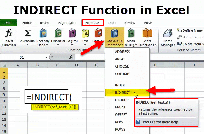
Understanding the Syntax of the INDIRECT Function
The basic syntax of the INDIRECT function in Excel is as follows:
excel
INDIRECT(ref_text, [a1])
ref_text: A string that contains the reference to a cell or range of cells. This reference can be to a single cell, a range of cells, or even a named range. The reference can be provided in the A1 style (e.g., “A1”) or the R1C1 style (e.g., “R1C1”).
[a1] (optional): This is a logical value (TRUE or FALSE) that specifies whether the reference style is A1 (TRUE) or R1C1 (FALSE). By default, this argument is set to TRUE, meaning Excel uses the A1 style unless otherwise specified.
The INDIRECT function can be used to reference cells or ranges that change dynamically. This makes it incredibly useful in scenarios where the exact cell or range reference might change based on the content of other cells or external factors.
Using INDIRECT to Reference Another Sheet
One of the most powerful applications of the INDIRECT function in Excel is the ability to reference a cell or range from another sheet. For example, suppose you have a workbook with multiple sheets, and you need to create a formula that refers to a specific cell on a different sheet. You could use the INDIRECT function to build that reference dynamically, even if the sheet name changes.
Consider the following example:
Let’s say you have two sheets in your workbook: Sheet1 and Sheet2. You want to reference cell A1 from Sheet2. You can use the following formula:
excel
=INDIRECT("Sheet2!A1")
This formula will return the value in cell A1 from Sheet2. If the name of Sheet2 changes, you can simply change the text inside the INDIRECT function, and the reference will update automatically.
In cases where the sheet name might change dynamically, you can use a cell reference to store the sheet name. For example:
excel
=INDIRECT(A1 & "!A1")
If cell A1 contains the name Sheet2, this formula will return the value from cell A1 in Sheet2. If the value in cell A1 changes to Sheet3, the reference will automatically update.
Advanced INDIRECT Function in Excel
While the INDIRECT function is often used in simple references, it can also be used in more advanced scenarios to create flexible and dynamic formulas. One of the most advanced ways to use the INDIRECT function is by referencing dynamic ranges, performing complex calculations, and using nested INDIRECT functions.
INDIRECT Function with Dynamic Ranges
The INDIRECT function can be particularly useful when working with ranges that may change dynamically based on user input or other data in the workbook. For example, you might have a list of numbers in a column, and you want to sum the values in a range of cells, but the exact range will change based on user input.
Suppose you have a workbook where the start and end rows of a range are defined in cells B1 and B2, respectively. You can use the INDIRECT function to reference this dynamic range as follows:
excel
=SUM(INDIRECT("A" & B1 & ":A" & B2))
In this formula, if the values in cells B1 and B2 change, the INDIRECT function will adjust the range that is being summed accordingly. This approach is especially useful when you don’t know the exact range beforehand and need to reference a range that changes dynamically.
Excel INDIRECT with R1C1 Reference Style
The R1C1 reference style is another way to reference cells in Excel. Instead of using the traditional A1 style (e.g., “A1”, “B3”), the R1C1 style uses numbers to represent both rows and columns. For example, “R1C1” refers to the cell in row 1, column 1, while “R3C2” refers to the cell in row 3, column 2.
The INDIRECT function can also be used with R1C1 references. To do so, you simply pass the R1C1 reference as text to the INDIRECT function, and it will return the corresponding cell value. For example:
excel
=INDIRECT("R1C1", FALSE)
This formula will return the value in the cell located at row 1, column 1, using the R1C1 style of referencing. When working with complex formulas or when trying to dynamically generate references, using R1C1 references can make the INDIRECT function even more powerful and flexible.
Nested INDIRECT Functions in Excel
Another advanced use of the INDIRECT function is the ability to nest multiple INDIRECT functions within a single formula. Nesting allows you to reference multiple ranges or even sheets within one formula, making it highly flexible.
Consider the following example, where you have two sheets: Sheet1 and Sheet2. Each sheet has a different range of data, and you want to dynamically switch between the ranges based on user input.
You can use a nested INDIRECT function to reference different ranges in the two sheets like so:
excel
=SUM(INDIRECT("Sheet" & A1 & "!A1:A10"))
In this formula, if the value in cell A1 is 1, the INDIRECT function will reference the range A1:A10 on Sheet1. If the value in A1 is 2, it will reference the range A1:A10 on Sheet2. This type of nesting can be extended to reference entire ranges, ranges on multiple sheets, or even dynamic cell references based on user input.
Excel INDIRECT and the SUM Function
The SUM function is one of the most commonly used functions in Excel, and it works seamlessly with the INDIRECT function to perform calculations on dynamic ranges. The INDIRECT function allows you to reference a range indirectly, and the SUM function can be used to add up the values in that range.
For example, let’s say you want to sum a range of cells that changes dynamically based on user input. If the start and end rows of the range are defined in cells B1 and B2, you can use the following formula:
excel
=SUM(INDIRECT("A" & B1 & ":A" & B2))
This formula will sum the values in column A, from the row specified in B1 to the row specified in B2. As the values in B1 and B2 change, the range being summed will update accordingly.
Conclusion
The INDIRECT function in Excel is a powerful tool that allows users to dynamically reference cells, ranges, and even sheets in their formulas. It is particularly useful when you need to create flexible and adaptable formulas that can adjust to changing data or user input. Whether you are working with dynamic ranges, referencing different sheets, or nesting multiple functions, the INDIRECT function offers countless possibilities for enhancing your Excel workflows.
By understanding its basic syntax and exploring advanced scenarios such as nested INDIRECT functions, R1C1 references, and using INDIRECT with the SUM function, you can unlock the full potential of this versatile Excel feature. With these tools in your Excel toolkit, you can create more powerful, adaptable, and efficient spreadsheets that can handle a wide range of tasks.
GetSPSSHelp is the best choice for mastering the INDIRECT function in Excel because of our expert guidance and student-focused approach. Our team simplifies complex concepts, providing clear, step-by-step instructions to help you create dynamic cell references effortlessly. We ensure accuracy, save time, and enhance your understanding of Excel. With affordable pricing, 24/7 support, and a commitment to quality, we make learning INDIRECT stress-free and effective. Whether you’re a beginner or advanced user, GetSPSSHelp empowers you to excel in data analysis. Trust us for reliable, professional assistance that boosts your skills and confidence!
Needs help with similar assignment?
We are available 24x7 to deliver the best services and assignment ready within 3-4 hours? Order a custom-written, plagiarism-free paper
https://getspsshelp.com/wp-content/uploads/2024/12/logo-8.webp00Besttutorhttps://getspsshelp.com/wp-content/uploads/2024/12/logo-8.webpBesttutor2025-01-31 07:32:062025-04-08 20:52:05The INDIRECT Function in Excel: A Comprehensive Overview|2025
Learn how to use the OFFSET function in Excel to dynamically reference data ranges and streamline your data analysis. Master this powerful tool for efficient workflows and reporting!
Excel is a powerful tool for data analysis and management, with a multitude of functions that simplify complex tasks. One of the most versatile functions in Excel is the OFFSET function, which allows users to create dynamic ranges, adjust data references, and improve overall spreadsheet flexibility. In this paper, we will delve into the OFFSET function in Excel, its benefits, how to use it with other functions like INDIRECT, and how to work with dynamic ranges. We will also explore examples and practical applications such as Excel SUM OFFSET dynamic range and Excel OFFSET MATCH.
Understanding the OFFSET Function in Excel
The OFFSET function in Excel is used to return a reference to a range that is a specified number of rows and columns from a starting cell or range. The syntax for the function is:
reference: The starting point, or base cell, from where the offset will be applied.
rows: The number of rows to move from the starting reference (can be positive or negative).
columns: The number of columns to move from the starting reference (can be positive or negative).
height (optional): The number of rows to return in the reference.
width (optional): The number of columns to return in the reference.
OFFSET Function in Excel Shortcut
While there isn’t a direct “shortcut” for entering the OFFSET function, the process is straightforward. To use the OFFSET function in Excel, you typically begin by selecting a cell, typing =OFFSET(), and filling in the required arguments. Once you become familiar with the function, entering it quickly becomes second nature. If you’re looking for a quicker way to reference cells in a dynamic range, utilizing Excel’s Name Manager to create defined names for your OFFSET ranges can save you time.
Excel OFFSET Dynamic Range
One of the most powerful uses of the OFFSET function is to create dynamic ranges. A dynamic range automatically adjusts when new data is added or removed. This is especially useful when working with large datasets or reports that frequently change. The OFFSET function can dynamically reference a range, ensuring your formulas always use the correct data without needing to manually update references.
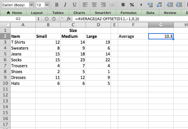
For example, suppose you have a dataset in cells A1:A10, and you want to create a dynamic range that expands as new data is added. The formula would look like:
swift
=OFFSET($A$1,0,0,COUNTA($A:$A),1)
Explanation:
The reference $A$1 is the starting point.
The rows argument is 0, meaning no offset from the starting point.
The columns argument is 0, meaning no horizontal shift.
COUNTA($A:$A) counts the number of non-empty cells in column A, thus setting the height of the range dynamically.
The width is 1, which means the range is just one column wide.
Now, when new data is added to column A, the dynamic range will automatically adjust to include the new rows.
Benefits of OFFSET Function in Excel
The OFFSET function in Excel offers numerous benefits that enhance spreadsheet functionality:
Dynamic Data Ranges: As demonstrated earlier, OFFSET can be used to create dynamic data ranges that update automatically. This is particularly useful for charts and tables that need to adjust as data changes.
Flexible Data Manipulation: OFFSET can be used to reference data that may not be in a fixed location. This is helpful when working with large datasets or when data is frequently updated.
Improved Formula Efficiency: Instead of manually adjusting cell references in formulas, OFFSET allows users to define flexible ranges that automatically update, improving the accuracy of calculations.
Better Data Analysis: By combining OFFSET with other functions like SUM, AVERAGE, and MATCH, you can create more complex and efficient formulas, allowing for deeper data analysis.
Using the INDIRECT and OFFSET Function in Excel
The INDIRECT function in Excel is another powerful tool that can be used in conjunction with OFFSET to enhance flexibility. The INDIRECT function returns a reference specified by a text string, meaning that you can use it to refer to dynamic ranges or cells. When combined with the OFFSET function, the two can be used to reference a range that is not statically defined but rather calculated through text strings.
For example, if you have a cell containing a reference to another cell (such as A1), and you want to use this reference dynamically in an OFFSET formula, you could combine INDIRECT and OFFSET like this:
less
=OFFSET(INDIRECT("A1"), 2, 3)
This formula will offset the reference from cell A1 by 2 rows down and 3 columns to the right. The INDIRECT function allows for dynamic referencing, meaning the formula can adjust as the reference changes.
Excel OFFSET from Current Cell
Another useful feature of the OFFSET function in Excel is its ability to reference a range from the current cell. This can be particularly handy when working with relative references and creating formulas that can be copied across multiple cells.
For example, if you want to sum the range of cells in the row directly beneath the current cell, you could use the following OFFSET formula:
INDIRECT(ADDRESS(ROW(),COLUMN())) gives the reference to the current cell.
1,0 tells Excel to move one row down from the current cell.
5,1 specifies that the range includes 5 rows and 1 column.
This formula will sum the five cells in the column directly below the current cell.
OFFSET Formula Example
Here’s an example of how you can use the OFFSET function in Excel for real-world applications:
Example: Calculating the Sum of a Dynamic Range
Suppose you have a table of sales data in column A, and you want to calculate the total sales for the last 5 rows of data. You can use the OFFSET function to create a dynamic range that automatically adjusts as new rows are added to the dataset:
less
=SUM(OFFSET(A1,COUNTA(A:A)-5,0,5,1))
Explanation:
A1 is the starting reference.
COUNTA(A:A)-5 moves the reference 5 rows before the last non-empty row in column A.
0,0 indicates no horizontal offset.
5,1 specifies a range of 5 rows and 1 column.
This formula will automatically sum the last 5 rows of data in column A as new rows are added.
Excel SUM(OFFSET Dynamic Range)
As shown in the example above, the SUM(OFFSET dynamic range) formula allows you to sum values from a range that dynamically adjusts as new data is added. This is particularly useful for financial or sales reports where the dataset grows over time.
For example, if you want to sum a range that starts from a fixed cell and extends based on the number of entries in another column, you could use:
swift
=SUM(OFFSET($A$1,0,0,COUNTA($B:$B),1))
Here, COUNTA($B:$B) counts the number of entries in column B, and the OFFSET function returns a sum of values from column A for the same number of rows.
Excel OFFSET MATCH
The OFFSET function combined with the MATCH function is another powerful feature in Excel. The MATCH function returns the relative position of a value in a range. When used with OFFSET, it allows you to find a specific value and create a dynamic reference to it.
For example, if you have a list of names in column A and their corresponding sales figures in column B, and you want to reference the sales figure for a specific name, you could use:
less
=OFFSET(A1,MATCH("John",A:A,0)-1,1)
Explanation:
MATCH("John",A:A,0) finds the row number where “John” is located in column A.
-1 adjusts the result to match the correct row relative to A1.
1 indicates that the sales figure is in the next column, column B.
This formula will return the sales figure for John, and it will adjust dynamically if the list is modified.
Conclusion
The OFFSET function in Excel is an invaluable tool that enhances the flexibility of spreadsheets, particularly when dealing with dynamic data and ranges. Whether you are creating dynamic ranges, using OFFSET with other functions like INDIRECT and MATCH, or applying it to more complex calculations like SUM, the OFFSET function offers a wealth of possibilities for data analysis and management. Mastering the OFFSET function is essential for anyone looking to improve their Excel skills and streamline their workflows.
GetSPSSHelp is the best choice for mastering the OFFSET function in Excel because of our expert guidance and student-focused approach. Our team simplifies complex concepts, providing clear, step-by-step instructions to help you dynamically reference data ranges effortlessly. We ensure accuracy, save time, and enhance your understanding of Excel. With affordable pricing, 24/7 support, and a commitment to quality, we make learning OFFSET stress-free and effective. Whether you’re a beginner or advanced user, GetSPSSHelp empowers you to excel in data analysis. Trust us for reliable, professional assistance that boosts your skills and confidence.
Needs help with similar assignment?
We are available 24x7 to deliver the best services and assignment ready within 3-4 hours? Order a custom-written, plagiarism-free paper
https://getspsshelp.com/wp-content/uploads/2024/12/logo-8.webp00Besttutorhttps://getspsshelp.com/wp-content/uploads/2024/12/logo-8.webpBesttutor2025-01-31 07:30:332025-02-15 05:26:35The OFFSET Function in Excel: A Comprehensive Guide|2025