The CHOOSE Function in Excel: An In-Depth Guide|2025
/in Advanced Excel Articles /by BesttutorLearn how to use the CHOOSE function in Excel to streamline data selection and improve your workflow. Master these essential tools for efficient data analysis and productivity!
The CHOOSE function in Excel is a powerful and versatile tool that allows users to select values from a list of options based on a given index or position. This function is commonly used in various scenarios to improve the efficiency of decision-making processes and streamline data manipulation. This paper will explore the CHOOSE function in Excel, its syntax, common use cases, and how to implement it in multiple scenarios, including working with multiple conditions, drop-down lists, arrays, and even combining it with other functions like VLOOKUP.
Understanding the CHOOSE Function
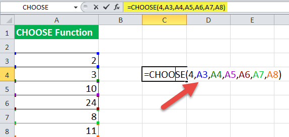
The CHOOSE function in Excel allows users to select one value from a list of options based on the position of the desired value. Its syntax is:
CHOOSE(index_num, value1, value2, ..., value_n)
- index_num: This is the position number of the value you want to choose from the list. It can be a static number or a dynamic reference, such as a result from another function.
- value1, value2, …, value_n: These are the possible values from which the CHOOSE function will pick. The function can accept up to 254 values.
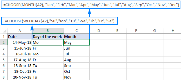
The function works by using the index number to select the corresponding value. If the index number is 1, the first value will be selected. If the index number is 2, the second value will be selected, and so on.
The CHOOSE Function Formula: An Example
To illustrate the use of the CHOOSE function, let’s consider a simple example. Suppose we have a list of products, and we want to select a product based on a given index number.
Example:
If you have a list of products like this:
- Product 1: Apples
- Product 2: Bananas
- Product 3: Oranges
The CHOOSE function can be used to select a product based on the index number:
=CHOOSE(2, "Apples", "Bananas", "Oranges")
This formula will return “Bananas” because the index number is 2, and Bananas is the second value in the list.
Multiple Conditions with the CHOOSE Function
While the basic CHOOSE function allows users to select values based on a single index number, it can be enhanced to handle multiple conditions. By combining the CHOOSE function with logical functions like IF or nested functions, users can evaluate multiple conditions and return different results based on those conditions.
Example: CHOOSE with Multiple Conditions
Suppose you are evaluating sales data for a team and want to assign a bonus based on performance, where:
- Sales above $10,000 = “High Bonus”
- Sales between $5,000 and $10,000 = “Medium Bonus”
- Sales below $5,000 = “Low Bonus”
You can combine the CHOOSE function with an IF statement to create a formula that evaluates the sales data and returns the corresponding bonus.
=CHOOSE(IF(A1>10000, 1, IF(A1>=5000, 2, 3)), "High Bonus", "Medium Bonus", "Low Bonus")
In this formula:
- If the sales (cell A1) are above $10,000, the first condition is met, and the function returns “High Bonus.”
- If the sales are between $5,000 and $10,000, the second condition is met, and it returns “Medium Bonus.”
- If the sales are below $5,000, the third condition is met, and the function returns “Low Bonus.”
This demonstrates how you can use the CHOOSE function to work with multiple conditions and handle more complex decision-making processes.
VLOOKUP with the CHOOSE Function in Excel
The CHOOSE function can also be combined with VLOOKUP to create more flexible and dynamic lookup operations. VLOOKUP typically allows users to search for a value in the first column of a table and return a corresponding value from another column. However, VLOOKUP is somewhat limited because it requires the lookup table to have a fixed structure. By combining VLOOKUP with the CHOOSE function, users can dynamically change the structure of the lookup table.
Example: VLOOKUP with CHOOSE
Let’s say you have a table that contains sales data for multiple regions, and you want to dynamically look up the sales for a specific region.
| Region | Sales |
|---|---|
| North | 2000 |
| South | 3000 |
| East | 4000 |
| West | 5000 |
Now, if you want to look up the sales for a specific region but the regions are listed in a different order or you want to look up data across multiple columns, you can use the CHOOSE function to reorder the columns dynamically.
=VLOOKUP("South", CHOOSE({1,2}, {"North","South","East","West"}, {2000, 3000, 4000, 5000}), 2, FALSE)
In this formula:
- The CHOOSE function is used to rearrange the columns of the table dynamically, making it possible to use VLOOKUP in scenarios where the order of columns is not fixed.
- The first argument of VLOOKUP is the lookup value (“South”).
- The second argument is the table array, which is dynamically created by CHOOSE.
- The third argument (2) specifies that we want to return the value in the second column of the dynamically created table.
This approach expands the flexibility of VLOOKUP, allowing you to modify the lookup structure without changing the original data.
CHOOSE Function Excel Scenarios
The CHOOSE function can be used in a variety of scenarios in Excel, especially when you need to select values or categories from a predefined list. Some common scenarios include:
- Selecting from Multiple Options: For example, selecting from different payment methods (Cash, Credit, Debit).
- Creating Custom Reports: By selecting different columns or rows of data based on user input, you can create customized reports.
- Dynamic Dashboards: The CHOOSE function is often used in dashboards to dynamically change the displayed information based on user input, such as choosing between different metrics like revenue, expenses, or profits.
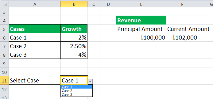
Excel CHOOSE Function Drop-Down List
One of the most practical uses of the CHOOSE function is in creating drop-down lists for data entry. The drop-down list allows users to select from a list of predefined options, reducing the risk of input errors.
Example: Drop-Down List with CHOOSE
Suppose you want to create a drop-down list that allows users to select the product category from a list of options. You can use the CHOOSE function to dynamically populate the list based on a user’s selection.
- Create a list of product categories (e.g., Electronics, Furniture, Clothing).
- Use the CHOOSE function to display the relevant product data for the selected category.
=CHOOSE(DropDownList, "Electronics", "Furniture", "Clothing")
When the user selects a category from the drop-down list, the CHOOSE function will return the corresponding value based on the selection.
Excel CHOOSE Function Array
The CHOOSE function can also be used with arrays to perform operations on multiple values at once. When you combine the CHOOSE function with arrays, you can create formulas that evaluate several sets of values and return the desired results.
Example: CHOOSE with Arrays
Suppose you want to sum values based on multiple criteria, where the values are selected from an array of options. You could use the CHOOSE function to return values from an array based on a dynamic condition.
=SUM(CHOOSE({1,2}, A1:A10, B1:B10))
This formula will sum the values from the array of columns A1:A10 and B1:B10, depending on the index provided.
Excel Formula to Choose Between Two Values
Another common scenario is using the CHOOSE function to select between two values based on a simple condition. This can be useful for binary decision-making processes.
Example: Choosing Between Two Values
=CHOOSE(IF(A1 > 1000, 1, 2), "High Value", "Low Value")
This formula will return “High Value” if the value in A1 is greater than 1000, and “Low Value” otherwise.

Conclusion
The CHOOSE function in Excel is an extremely useful tool that allows users to select values dynamically based on an index or condition. It can be used in various scenarios, from simple lookups to complex decision-making processes, especially when combined with other Excel functions like VLOOKUP and IF. By understanding its syntax and potential applications, users can significantly enhance their data manipulation and reporting capabilities in Excel. Whether you’re working with drop-down lists, arrays, or conditional statements, the CHOOSE function is a versatile and powerful tool to add to your Excel toolkit.
GetSPSSHelp is the best choice for mastering the CHOOSE function in Excel because of our expert guidance and student-focused approach. Our team simplifies complex concepts, providing clear, step-by-step instructions to help you select and retrieve data effortlessly. We ensure accuracy, save time, and enhance your understanding of Excel. With affordable pricing, 24/7 support, and a commitment to quality, we make learning CHOOSE stress-free and effective. Whether you’re a beginner or advanced user, GetSPSSHelp empowers you to excel in data analysis. Trust us for reliable, professional assistance that boosts your skills and confidence.
Needs help with similar assignment?
We are available 24x7 to deliver the best services and assignment ready within 3-4 hours? Order a custom-written, plagiarism-free paper


:max_bytes(150000):strip_icc()/date-function-example-e60abfc348994855bbc30338e26b5cad.png)