Common Stata Errors and How to Fix Them|2025

Common Stata Errors and How to Fix Them offers solutions to frequent issues encountered in Stata. Learn how to troubleshoot, resolve errors, and improve your data analysis workflow with expert tips

Stata is a powerful statistical software used by researchers, data analysts, and statisticians to manage, analyze, and visualize data. Despite its robustness, users often encounter errors that can disrupt their workflow. These errors can stem from various sources such as system issues, software configuration, or mistakes in the code. In this paper, we will examine some of the most common Stata errors, their potential causes, and how to fix them. The errors covered include issues with Stata updates, I/O problems, missing variables, and Java installation issues.

Common Stata Errors and How to Fix Them

Stata Error: “Stata did not respond or is not a valid update site”

This error typically occurs when users try to update Stata, and the software is unable to connect to the Stata website or another update source. The causes can vary but often include issues with Internet connectivity or Stata’s configuration settings.

Causes:

  • Internet connectivity issues: Stata requires an active internet connection to update. If there is no access to the internet, the update process will fail.
  • Stata Internet settings: Incorrect or misconfigured internet settings within Stata can prevent it from accessing the update site.
  • Firewall or proxy interference: A firewall or proxy server may block Stata from accessing the update server.

How to Fix It:

  • Check Internet connection: Ensure that your computer has an active internet connection. Try browsing the web or using other online services to confirm that the internet is working.
  • Verify Stata’s Internet settings: You can check Stata’s Internet settings by typing the following command:
    stata
    set internet on

    This command ensures that Stata can access the internet. If you are using a proxy server, you may need to configure Stata’s proxy settings:

    stata
    set httpproxy <proxy_address>
    set httpsproxy <proxy_address>
  • Disable firewall or adjust settings: Check your firewall settings to ensure it is not blocking Stata’s connection to the update site. You may need to allow Stata to access the internet or temporarily disable the firewall.

Stata Error Codes: Understanding and Troubleshooting

Stata provides a range of error codes that help users diagnose issues within their scripts or commands. These codes typically consist of a number followed by an error message. Some common Stata error codes include:

  • r(198): This error occurs when a command fails to run due to insufficient memory.
  • r(111): This error indicates that the file specified for input or output cannot be opened.
  • r(2000): This error is usually caused by an invalid command syntax.

How to Fix It:

  • r(198): Increase memory allocation by using the set memory command. For example, to allocate 1GB of memory, you can type:
    stata
    set memory 1g
  • r(111): Ensure that the file path is correct and that the file is not in use by another program.
  • r(2000): Double-check the syntax for your command, making sure that all required arguments and options are included.

Common Stata Errors and How to Fix Them

Java Installation Not Found in Stata

Some advanced Stata features, such as web scraping, require Java to be installed on your system. If Java is not installed or Stata cannot locate it, you may encounter an error message saying that “Java installation not found.”

Causes:

  • Missing Java installation: If Java is not installed on your computer, Stata will be unable to use Java-based features.
  • Incorrect Java path: Stata might not be able to find the Java installation if it is not properly configured or if the environment variables are incorrect.

How to Fix It:

  • Install Java: Ensure that you have Java installed on your system. You can download and install Java from the official Java website.
  • Set Java path in Stata: If Java is installed but Stata cannot detect it, you may need to specify the location of the Java installation in Stata. You can do this by typing the following command in the Stata command window:
    stata
    set java_path "C:\Program Files\Java\jre1.8.0_171"

    Replace the path with the actual location of your Java installation.

Stata I/O Error: File Cannot Be Opened

I/O errors in Stata typically occur when trying to read from or write to a file. These errors can prevent data from being imported or exported correctly.

Causes:

  • File is already in use: If the file is currently being used by another program, Stata may be unable to access it.
  • File permissions: Insufficient permissions can prevent Stata from opening or saving the file.
  • Corrupted file: If the file is damaged or corrupted, Stata may not be able to read or write data.

How to Fix It:

  • Close other programs: Make sure the file is not open in another application (e.g., Excel, Notepad).
  • Check file permissions: Verify that you have the appropriate read and write permissions for the file. If necessary, change the file permissions or move it to a directory where you have full access.
  • Try opening the file in another program: If the file is corrupted, try opening it in a different program (e.g., Excel) to check if the data is still intact.

Common Stata Errors and How to Fix Them

Stata Set Trace On

The set trace on command is a powerful debugging tool in Stata. It displays detailed information about the execution of commands, including each line of code that is executed. This can help users identify where errors are occurring in their scripts.

Causes:

  • Debugging complex code: When you have a complex script, it can be difficult to pinpoint where errors are happening. Using set trace on helps you trace through the code step by step.
  • Verbose output: The trace command generates a lot of output, which can be overwhelming if you’re not used to it.

How to Use It:

  • Activate trace: To activate tracing, type:
    stata
    set trace on

    This will show you detailed output as the commands are executed.

  • Turn off trace: Once you have identified the error, you can turn off tracing by typing:
    stata
    set trace off

Variable Not Found in Stata

One of the most common errors in Stata occurs when you attempt to use a variable that does not exist in your dataset. The error message usually reads: “variable not found.”

Causes:

  • Incorrect variable name: If you mistype the name of the variable, Stata will not recognize it.
  • Dropped or missing variable: The variable may have been dropped or may not exist in the current dataset.
  • Wrong dataset: If you’re working with multiple datasets, it’s possible that the variable exists in another dataset but not the one currently loaded in memory.

How to Fix It:

  • Check variable name: Double-check the variable name for typos. You can list all variables in the dataset by typing:
    stata
    describe
  • Verify dataset: Ensure that the correct dataset is loaded. If you’re working with multiple datasets, you may need to load the appropriate one using the use command:
    stata
    use dataset_name
  • Create or restore variable: If the variable has been dropped, you may need to recreate it or restore it from a previous version of the dataset.

Common Stata Errors and How to Fix Them

Stata Internet Settings

Stata’s internet settings control how the software interacts with the web. Misconfigured settings can lead to various errors, particularly when trying to access online resources or update Stata.

Causes:

  • Firewall or network restrictions: Stata may not be able to access the internet due to firewall restrictions or network configurations.
  • Incorrect proxy settings: If you are behind a proxy server, incorrect proxy settings can block Stata’s internet access.

How to Fix It:

  • Check firewall settings: Make sure that Stata is not being blocked by your firewall. You may need to adjust your firewall rules to allow Stata to access the internet.
  • Configure proxy settings: If you are using a proxy, make sure Stata is configured to use it. You can set the proxy settings by typing:
    stata
    set httpproxy proxy_address
    set httpsproxy proxy_address

Common Stata Errors and How to Fix Them

Conclusion

Stata is an incredibly powerful statistical tool, but like any software, it can be prone to errors. Understanding common Stata errors such as connectivity issues, I/O errors, missing variables, and Java-related problems is essential for troubleshooting and ensuring smooth operations. By diagnosing the cause of these errors and applying the appropriate solutions, users can quickly resolve issues and get back to their analysis. Moreover, utilizing debugging tools like set trace on can help streamline the debugging process. With these strategies, users can make the most out of Stata’s capabilities and minimize disruptions in their workflow.

GetSPSSHelp is the best website for “Common Stata Errors and How to Fix Them” because it provides expert advice on troubleshooting and resolving frequent Stata issues. The platform offers clear, step-by-step solutions for a wide range of errors, helping users quickly get back on track with their data analysis. GetSPSSHelp’s team of professionals is dedicated to providing personalized support, ensuring that each user can efficiently fix their Stata problems. With affordable pricing and high-quality resources, it is the go-to resource for anyone seeking to improve their Stata skills. Additionally, 24/7 customer support ensures prompt assistance, making GetSPSSHelp a trusted choice for resolving Stata errors.

Needs help with similar assignment?

We are available 24x7 to deliver the best services and assignment ready within 3-4 hours? Order a custom-written, plagiarism-free paper

Get Answer Over WhatsApp Order Paper Now

How to Interpret Stata Output: A Comprehensive Guide|2025

How to Interpret Stata Output: A Comprehensive Guide offers detailed instructions on understanding and interpreting Stata results. Learn how to analyze statistical outputs and draw accurate conclusions from your data.

Stata is a widely used statistical software that provides a robust environment for data analysis, particularly for regression analyses. Understanding how to interpret Stata’s regression output is crucial for making informed conclusions and reporting research findings. This paper will guide you through interpreting different aspects of Stata output, particularly focusing on linear regression, dummy variables, and logistic regression. It will also cover concepts such as p-values, t-statistics, and how to approach Stata regression output tables. Additionally, relevant resources like the Stata regression output interpretation PDF will be referenced for further reading.

How to Interpret Stata Output

Introduction

Stata’s regression output can be complex and dense, especially when dealing with different types of regression models. However, with a systematic approach, understanding the output becomes manageable. By interpreting the coefficients, p-values, t-statistics, R-squared values, and other relevant statistics, you can draw meaningful conclusions from your data. In this guide, we will walk you through key components of Stata output and provide step-by-step instructions for interpreting the results in multiple linear regression and logistic regression, as well as how to interpret dummy variables in regression models.

Overview of Stata Output

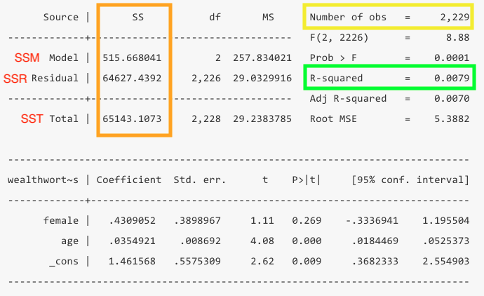
Before diving into interpretation, it’s important to understand the structure of the output that Stata generates when you run a regression. The output typically consists of several tables:

  • Regression Coefficients Table: Contains the estimated coefficients, standard errors, t-statistics, p-values, and confidence intervals for each predictor variable.
  • Model Summary: Includes R-squared, adjusted R-squared, F-statistic, and the p-value associated with the F-test.
  • Diagnostic Statistics: Such as residuals, multicollinearity statistics (e.g., Variance Inflation Factor), and others depending on the type of regression.

The format of this output may vary depending on the type of regression analysis (e.g., linear or logistic), but understanding these core tables is essential for any interpretation.

Multiple Linear Regression Stata Output Interpretation

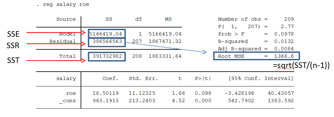
Let’s begin with multiple linear regression. In this case, the dependent variable is continuous, and you are examining the relationship between it and several independent variables. Once the regression command is executed in Stata, the regression output will look something like this:

. regress y x1 x2 x3

This generates an output with the following components:

  • Coef. (Coefficient): This is the estimated effect of each independent variable on the dependent variable. For example, if the coefficient for x1 is 3.5, this means that for every one-unit increase in x1, the dependent variable y is expected to increase by 3.5 units, holding all other variables constant.
  • Standard Error: This value tells you about the precision of the coefficient estimate. A smaller standard error indicates more precise estimates. The standard error can be used to construct confidence intervals for the coefficients.
  • t-statistic: This statistic tests whether the coefficient is significantly different from zero. It is calculated by dividing the coefficient by its standard error. A larger absolute t-statistic indicates stronger evidence against the null hypothesis that the coefficient is zero.
  • p-value: The p-value indicates the probability of observing a t-statistic as extreme as the one calculated, under the assumption that the null hypothesis (coefficient = 0) is true. A common threshold for significance is 0.05, meaning that if the p-value is less than 0.05, you can reject the null hypothesis and conclude that the variable has a significant effect on the dependent variable.
  • R-squared: This statistic measures the proportion of variance in the dependent variable that is explained by the independent variables. A higher R-squared means a better fit of the model to the data.

Example output for a multiple regression analysis:

Variable Coefficient Std. Error t-statistic p-value
x1 3.5 1.2 2.92 0.004
x2 -0.5 0.3 -1.67 0.097
x3 1.0 0.5 2.00 0.047

In this example:

  • The coefficient for x1 is 3.5, meaning that as x1 increases by one unit, y increases by 3.5 units. The p-value is 0.004, indicating statistical significance at the 5% level.
  • The coefficient for x2 is -0.5, but its p-value (0.097) is above 0.05, meaning this variable is not statistically significant at the 5% level.
  • The coefficient for x3 is 1.0, and the p-value (0.047) shows that it is statistically significant.

The Adjusted R-squared provides a more accurate measure of model fit, especially when multiple predictors are included in the model.

How to Interpret Stata Output

How to Interpret Dummy Variables in Regression Stata

Dummy variables are used in regression models to represent categorical variables. Stata automatically generates a baseline category and assigns 1 or 0 to the remaining categories based on the presence or absence of a particular characteristic.

For instance, if you include a variable gender in your regression model with values 0 for male and 1 for female, Stata will treat this as a dummy variable. The output might look something like this:

Variable Coefficient Std. Error t-statistic p-value
Male (0) 0.0 0.0
Female (1) 2.5 1.1 2.27 0.024

In this example:

  • The coefficient for Female (1) is 2.5, meaning that being female is associated with an increase of 2.5 units in the dependent variable, relative to the male baseline (when Male (0) is used as the reference category).
  • If the p-value for Female (1) is less than 0.05, as in this case, you would conclude that gender has a statistically significant effect on the dependent variable.

Logistic Regression Stata Interpretation

Logistic regression is used when the dependent variable is binary (e.g., yes/no, 0/1). The output from logistic regression is somewhat different from linear regression because the coefficients represent the log-odds of the dependent variable occurring rather than the expected change in the dependent variable.

Example logistic regression output:

. logit y x1 x2 x3
Variable Coefficient Std. Error z-statistic p-value
x1 0.85 0.3 2.83 0.005
x2 -0.45 0.2 -2.25 0.024
x3 0.20 0.1 2.00 0.045

For logistic regression, the interpretation is based on the odds ratio, which is calculated by exponentiating the coefficient. For example:

  • The odds ratio for x1 is exp(0.85) = 2.34, meaning that for each one-unit increase in x1, the odds of y occurring (relative to not occurring) increase by a factor of 2.34.

Thus, logistic regression output interpretation focuses on the odds of the outcome variable occurring, as opposed to the direct effect seen in linear regression.

How to Interpret Stata Output

Understanding the p-value from the t-statistic in Stata

In any regression analysis, the p-value is a crucial statistic. It tells you whether the observed relationship between the independent and dependent variables is statistically significant. For a given t-statistic, the p-value is computed to assess whether the coefficient is significantly different from zero.

  • If the p-value is smaller than 0.05, you reject the null hypothesis, meaning the predictor variable is statistically significant.
  • If the p-value is greater than 0.05, you fail to reject the null hypothesis, meaning the predictor variable is not statistically significant.

How to Interpret Stata Output

Conclusion

Interpreting Stata’s regression output requires a clear understanding of key statistics, such as coefficients, p-values, t-statistics, and R-squared. By carefully analyzing these components, you can draw meaningful conclusions from your regression analysis. Whether you are dealing with multiple linear regression, logistic regression, or dummy variables, Stata provides all the necessary information to interpret the results and make informed decisions. For further details, resources like Stata regression output interpretation PDF can provide more in-depth guidance.

In conclusion, understanding how to interpret regression results in Stata is a vital skill for any researcher or data analyst. The process involves examining coefficients, checking statistical significance via p-values, and understanding model fit. With this knowledge, you can confidently use Stata to analyze your data and draw insightful conclusions.

GetSPSSHelp is the best website for “How to Interpret Stata Output: A Comprehensive Guide” because it provides expert guidance on understanding and analyzing Stata results. The platform breaks down complex statistical outputs into simple, actionable insights, making it easier to interpret data accurately. GetSPSSHelp offers personalized support, ensuring that users can apply Stata outputs effectively to their research and analysis. With affordable pricing and high-quality resources, it is the ideal choice for mastering Stata output interpretation. Additionally, 24/7 customer support ensures timely assistance, making GetSPSSHelp a trusted resource for anyone looking to understand Stata output.

Needs help with similar assignment?

We are available 24x7 to deliver the best services and assignment ready within 3-4 hours? Order a custom-written, plagiarism-free paper
Get Answer Over WhatsApp Order Paper Now

How to Install and Use Stata Packages: A Comprehensive Guide|2025

How to Install and Use Stata Packages: A Comprehensive Guide provides clear instructions on installing and utilizing Stata packages. Learn how to expand Stata’s functionality with step-by-step guidance for beginners and advanced users alike.

Stata is a powerful software used for data analysis, statistical modeling, and graphics. One of the key features of Stata is its extensibility through the use of packages. These packages are collections of commands and routines created by other users or developers, which extend Stata’s functionality and allow you to perform tasks that might not be available with the standard installation.

This paper will provide a detailed guide on how to install and use Stata packages, covering everything from using the ssc install command to manually installing packages, and how to manage installed packages. By the end of this guide, you will be able to install, use, and uninstall Stata packages effectively.

How to Install and Use Stata Packages

What Are Stata Packages?

Stata packages are additional components or routines that can be installed to extend Stata’s functionality. These packages are typically written in Stata’s programming language and can perform specific tasks that users find useful for their data analysis or research. Stata’s package system allows users to share their work, making it easier for others to implement advanced features without having to reprogram them.

Packages in Stata can range from simple commands that automate repetitive tasks to complex functions that provide cutting-edge statistical techniques. Stata provides an infrastructure for discovering, installing, and managing these packages directly from within the software.

How to Install and Use Stata Packages

There are several ways to install Stata packages, and the method you choose will depend on your needs. Below is a breakdown of the most common methods for installing and using Stata packages.

Installing Stata Packages Using the ssc install Command

The easiest and most common method for installing Stata packages is through the ssc install command. This command installs packages directly from the Statistical Software Components (SSC) archive, a public repository of Stata packages.

To install a package from the SSC archive, you simply use the ssc install command followed by the name of the package. For example:

stata
ssc install package_name

Where package_name is the name of the Stata package you want to install. When you execute this command, Stata will search the SSC archive, download the package, and install it automatically. You can then use the installed package in your session.

Example

If you want to install the package outreg2, which is used for creating tables of regression results, you would use the following command:

stata
ssc install outreg2

Stata will download and install the package, after which you can use the outreg2 command in your analysis.

Installing Stata Packages Manually

In some cases, you may want to install a Stata package manually. This is typically the case when a package is not available through the SSC archive or when you need to install a package from a custom source, such as a ZIP file or a GitHub repository.

To install a package manually, you need to follow these steps:

  1. Download the Package: First, you need to download the package files. These could be in the form of a .zip file or individual .ado and .hlp files.
  2. Place the Files in the Correct Directory: After downloading, place the package files in Stata’s “ado” directory. This directory is where Stata looks for user-installed programs. You can find this directory by typing the following command in Stata:
    stata
    sysdir

    This will display the paths of Stata’s system directories, including the “ado” directory. Once you know where the directory is, you can copy the package files there.

  3. Refresh Stata: After the files are placed in the appropriate directory, you may need to refresh Stata to recognize the new package. To do this, use the following command:
    stata
    adopath + "path_to_your_package"

    Replace "path_to_your_package" with the path to the directory containing the package. This command adds the directory to Stata’s search path, allowing Stata to find and use the package.

  4. Test the Installation: Finally, test the installation by running a command from the package. If the package was installed correctly, Stata should recognize the command and execute it without any errors.

How to Install and Use Stata Packages

Stata Packages List and Finding New Packages

To explore and find new Stata packages, you can search the SSC archive or other sources. Stata provides several commands for discovering available packages.

Using the findit Command

The findit command in Stata is an easy way to search for packages or commands within Stata’s repositories. For example, if you are looking for packages related to regression, you can type:

stata
findit regression

This will return a list of packages, resources, and documentation related to regression analysis.

Stata Package Lists and Repositories

Aside from the SSC archive, there are other sources where Stata packages are available, such as:

  • Stata Journal: The Stata Journal publishes packages as part of its research articles.
  • GitHub: Many developers share Stata packages on GitHub, where you can download and install them.
  • Other Stata-Related Websites: There are other websites that host Stata packages, often focused on specific areas of research.

If you’re unsure about where to find a particular package, using findit is the best way to start.

Uninstalling Stata Packages

If you no longer need a Stata package, you can uninstall it to free up space and reduce clutter. Stata makes it easy to uninstall packages with the ado uninstall command. To uninstall a package, use the following command:

stata
ado uninstall package_name

Where package_name is the name of the package you wish to uninstall. After executing this command, Stata will remove the package from the system.

Example

To uninstall the outreg2 package, you would use:

stata
ado uninstall outreg2

This command will remove the package from Stata, and you will no longer be able to use the outreg2 command unless you reinstall it.

How to Install and Use Stata Packages

How to Manage Stata Packages

Managing installed Stata packages involves keeping track of the packages you have installed and ensuring they are up to date. Stata provides several commands for managing installed packages.

Listing Installed Packages

To see a list of all installed packages, you can use the adopath command. This command shows you the directories where Stata is looking for user-installed programs, and you can check which packages are in those directories. For example:

stata
adopath

This will display the directories, including the location of installed packages. You can also list packages that are available in your current session by checking the “ado” folder in the directory where you installed them.

Updating Packages

Stata allows you to update installed packages to the latest version. To update a package, you can use the following command:

stata
ssc install package_name, replace

This command will check for any updates to the specified package. If a newer version is available, Stata will replace the old version with the new one.

Stata 17 Free Download and Licensing

Stata 17, the latest version of the software, includes several new features and improvements. While Stata is not free software, you can download a trial version of Stata from the official website. To obtain the free trial version of Stata, visit the Stata download page, where you can choose to download a trial version for your platform. The trial version allows you to explore Stata’s capabilities for a limited period before committing to a license.

Stata offers various licensing options, including student, academic, and commercial licenses. Each type of license has different pricing, and you can select the one that fits your needs.

How to Install and Use Stata Packages

Conclusion

Installing and using Stata packages is a fundamental part of extending the software’s functionality and performing advanced statistical analyses. Whether you use the ssc install command to install packages from the SSC archive, install them manually, or manage your installed packages, Stata provides a robust system for working with third-party commands and routines.

By following the steps outlined in this paper, you can easily install, use, and manage Stata packages, enhancing your analytical capabilities. Additionally, understanding how to update and uninstall packages ensures that your Stata environment remains clean and efficient.

Stata’s ability to integrate user-contributed packages makes it an incredibly powerful tool for researchers, analysts, and statisticians. The diverse range of available packages means that no matter your area of interest, you can likely find a package that suits your needs.

By exploring the available Stata packages, you can dramatically improve your workflow, saving time and effort while gaining access to more advanced statistical methods.

Needs help with similar assignment?

We are available 24x7 to deliver the best services and assignment ready within 3-4 hours? Order a custom-written, plagiarism-free paper
Get Answer Over WhatsApp Order Paper Now

How to Perform Survival Analysis in Stata|2025

How to Perform Survival Analysis in Stata provides a comprehensive guide to conducting survival analysis using Stata. Learn essential techniques, commands, and interpretation methods for analyzing time-to-event data.

Introduction

Survival analysis is a branch of statistics that focuses on the analysis of time-to-event data. The time-to-event variable represents the time until a certain event of interest occurs, such as the failure of a machine, the occurrence of a medical event, or the time until a customer churns. In this paper, we will focus on how to perform survival analysis in Stata, one of the most popular statistical software programs used for data analysis.

Survival analysis involves the use of specialized statistical techniques to estimate the time until an event occurs and to examine the factors that may influence this time. Stata provides a comprehensive set of tools for performing survival analysis, from basic descriptive statistics to advanced models, such as Cox proportional hazards regression. We will explore the process of conducting survival analysis in Stata, using different types of data, model specifications, and Stata commands.

We will cover topics such as discrete-time survival analysis, how to handle censored data, and interpreting the results from Stata output. Additionally, we will look at specific resources like the Stata survival analysis manual, and how to use documents such as PDFs and PowerPoint presentations to learn about survival analysis in Stata.

How to Perform Survival Analysis in Stata

Overview of Survival Analysis

Survival analysis is used in many disciplines, such as medicine, engineering, and economics, to study the time until a specific event occurs. This time is often referred to as “survival time,” and the goal of survival analysis is to estimate the distribution of survival times, assess risk factors that might influence these times, and predict future survival outcomes.

There are several important concepts in survival analysis:

  • Censoring: Censoring occurs when the event of interest has not occurred by the end of the study or when the participant is lost to follow-up. This type of data can be challenging to analyze because we only have partial information about the event time.
  • Survival Function (S(t)): The survival function is the probability that the event of interest has not occurred by a certain time. It is typically estimated using Kaplan-Meier curves.
  • Hazard Function (h(t)): The hazard function describes the rate at which events occur over time. The hazard can vary over time and is often used in Cox regression models.
  • Cox Proportional Hazards Model: This is one of the most widely used models in survival analysis. It estimates the effect of predictor variables on the hazard rate, assuming that the effect of the covariates is constant over time.

Getting Started with Stata for Survival Analysis

To perform survival analysis in Stata, you first need to have the relevant data set that contains time-to-event information. This data typically includes a variable for survival time, an indicator for whether the event occurred, and other covariates that may affect survival.

Stata’s survival analysis commands are designed to handle different types of survival data, including right-censored data, left-censored data, and interval-censored data.

Data Setup for Survival Analysis

In Stata, survival time is often represented in a variable, say time, and the censoring indicator is represented as a variable, say status, where:

  • status = 1 indicates that the event of interest has occurred.
  • status = 0 indicates that the event was censored (i.e., the subject was lost to follow-up or the study ended before the event occurred).

To prepare your data for survival analysis in Stata, you need to declare the survival time and censoring variables using the stset command. For example:

stata
stset timevar, failure(statusvar)

In this case, timevar is the variable that contains the time until the event, and statusvar is the variable indicating whether the event occurred.

How to Perform Survival Analysis in Stata

Basic Survival Analysis Techniques in Stata

Kaplan-Meier Estimator

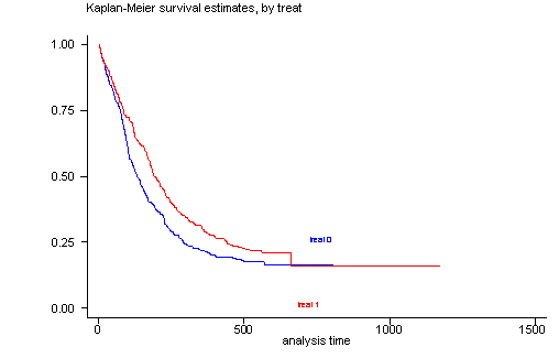
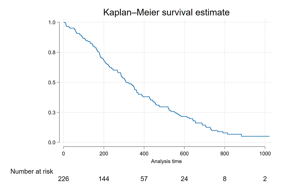
One of the most common techniques for survival analysis is the Kaplan-Meier estimator, which is used to estimate the survival function. The Kaplan-Meier curve shows the probability of survival over time, considering censoring.

To generate the Kaplan-Meier survival curve in Stata, you can use the following commands:

stata
sts list
sts graph

The sts list command provides a table of the survival function at different time points, and sts graph produces the Kaplan-Meier plot.

Log-Rank Test

The log-rank test is used to compare the survival distributions between two or more groups. For example, you may want to compare the survival times of two different treatment groups.

To perform a log-rank test in Stata, use:

stata
sts test groupvar

This command tests whether the survival curves for different groups (defined by groupvar) are statistically significantly different.

How to Perform Survival Analysis in Stata

Cox Proportional Hazards Model in Stata

The Cox proportional hazards model is a popular method for modeling survival data. It is used to assess the effect of explanatory variables (covariates) on the hazard rate, assuming that the effect of covariates is proportional over time.

To run a Cox regression in Stata, use the stcox command:

stata
stcox var1 var2 var3

Here, var1, var2, and var3 are the covariates you want to include in the model. The coefficients estimated from this model can be interpreted as the effect of each covariate on the hazard rate.

Discrete-Time Survival Analysis

In some cases, it may be necessary to perform discrete-time survival analysis, particularly when the survival times are measured in discrete time intervals (e.g., years, months). Stata provides a way to perform discrete-time survival analysis using logistic regression models.

The stset command is used to declare the data for discrete-time analysis:

stata
stset timevar, id(idvar) failure(statusvar) scale(1)

Then, you can use a logistic regression model for discrete-time survival analysis:

stata
logit statusvar var1 var2 var3

This will provide the odds of the event occurring, given the covariates.

How to Perform Survival Analysis in Stata

Handling Censoring in Stata

Censoring is an inherent feature of survival data. Stata provides commands and techniques to properly handle censored observations during analysis.

The key command to handle censoring is stset, which designates the failure indicator variable (status) and the survival time variable. The command takes care of censoring when estimating survival functions and hazards.

For instance, when performing a Cox regression, the status variable ensures that Stata only considers non-censored observations when computing hazard ratios.

Survival Analysis Example in Stata

Let’s go through an example of performing survival analysis in Stata with a hypothetical dataset. Suppose you have a dataset of patients undergoing a treatment, and you want to analyze the time until they experience a specific medical event (e.g., heart attack) while considering the impact of various covariates, such as age and gender.

  1. Loading the data: First, you load the dataset into Stata:
    stata
    use heart_disease_data.dta
  2. Setting up the survival data: You declare the survival time and censoring variables using stset:
    stata
    stset time_to_event, failure(event_occurred)
  3. Generating the Kaplan-Meier curve: To generate the Kaplan-Meier survival curve for the whole sample:
    stata
    sts graph
  4. Performing Cox regression: To analyze the effect of age and gender on the hazard of experiencing the event:
    stata
    stcox age gender

    This will provide you with hazard ratios for each covariate.

Useful Resources for Learning Survival Analysis in Stata

Several resources can assist you in performing survival analysis in Stata. These include:

  • An Introduction to Survival Analysis Using Stata (PDF): A comprehensive guide that introduces survival analysis methods and how to perform them in Stata.
  • Stata Survival Analysis Manual: This is the official manual that provides detailed instructions on all Stata survival analysis commands, from Kaplan-Meier estimators to Cox regression.
  • How to Perform Survival Analysis in Stata PPT: A PowerPoint presentation that summarizes key survival analysis techniques in Stata. This is useful for learning the basics and for classroom instruction.
  • Stata Survival Analysis Example: Stata’s website and various tutorials often provide practical examples and case studies to help you understand how to apply survival analysis in real-world scenarios.
  • Survival Analysis Stata UCLA: UCLA’s Institute for Digital Research and Education provides online tutorials and code for performing survival analysis in Stata. This is a great resource for learning how to perform various survival analysis techniques.

How to Perform Survival Analysis in Stata

Conclusion

Survival analysis is an essential tool for understanding time-to-event data. Stata offers a robust set of commands and techniques to perform survival analysis, whether you’re conducting a basic Kaplan-Meier analysis or using advanced regression models like Cox proportional hazards. By following the steps outlined in this paper and leveraging resources such as the Stata survival analysis manual and online tutorials, you can efficiently perform survival analysis in Stata and interpret the results to make informed decisions based on time-to-event data.

Needs help with similar assignment?

We are available 24x7 to deliver the best services and assignment ready within 3-4 hours? Order a custom-written, plagiarism-free paper

Get Answer Over WhatsApp Order Paper Now

Step-by-Step Guide to Data Visualization in Stata|2025

Step-by-Step Guide to Data Visualization in Stata teaches you how to create clear, impactful visualizations. Learn how to use Stata’s powerful tools for charts, graphs, and data presentation in this detailed tutorial.

Introduction

Data visualization is an essential aspect of data analysis as it allows researchers, analysts, and data scientists to communicate complex data in a more understandable, concise, and accessible way. Stata, a powerful software used for statistics and data management, offers a wide range of tools for creating visual representations of data, including graphs, charts, and plots. In this guide, we will provide a detailed step-by-step approach to data visualization in Stata, exploring the commands and techniques necessary to create effective and meaningful visualizations.

This tutorial assumes that the user has some basic knowledge of Stata and statistical analysis, but even beginners can follow along as we introduce fundamental concepts, commands, and strategies for producing various types of visualizations.

Throughout this guide, we will reference key terms such as “Data analysis using Stata PDF,” “An Introduction to statistics and data analysis using Stata PDF,” “How to use Stata for data analysis,” “Stata questions and answers PDF,” “Stata commands PDF,” “STATA data analysis examples,” and “Data analysis using Stata, third edition PDF.” These references will provide supplementary resources to deepen your understanding and enhance your learning experience.

Data Visualization in Stata

Getting Started with Stata for Data Visualization

Before diving into the details of creating data visualizations, it is essential to understand the foundational aspects of using Stata for data analysis and visualization.

  • Installing Stata: To begin, ensure that you have Stata installed on your computer. If you are new to Stata, you can find various installation guides and support on the Stata website. There are several versions available, including Stata/IC, Stata/SE, and Stata/MP, each offering varying levels of capacity based on the size of your data.
  • Setting up Your Data: A crucial first step is to load the data into Stata. If you are working with a CSV or Excel file, you can import it using commands like:
    stata
    import excel "your_data.xlsx", clear

    or

    stata
    import delimited "your_data.csv", clear

    Once the data is loaded, it’s important to inspect it using the list or browse command to check the structure and ensure there are no missing or incorrect values.

Basic Visualization Techniques in Stata

Stata offers an array of basic graphing capabilities, such as bar graphs, line graphs, scatter plots, and histograms. Here’s a rundown of how to create each of these fundamental visualizations:

  • Histograms: To visualize the distribution of a continuous variable, a histogram is a simple yet effective choice. Use the following command:
    stata
    histogram varname

    This will create a histogram of the variable varname. You can adjust the number of bins or add additional options to customize the appearance of the histogram.

  • Scatter Plots: Scatter plots are ideal for displaying the relationship between two continuous variables. The basic command for creating a scatter plot is:
    stata
    scatter var1 var2

    This will plot var1 on the x-axis and var2 on the y-axis. You can enhance the plot by adding options for colors, markers, or fitting a regression line.

  • Line Graphs: Line graphs are great for showing trends over time. To create a simple line graph, use:
    stata
    twoway (line var1 var2)

    This will plot a line representing var1 against var2. Adjustments can be made for more complex visualizations, such as multiple lines or adding labels.

  • Bar Charts: Bar charts are useful for displaying categorical data. The command to create a basic bar chart is:
    stata
    graph bar varname, over(categorical_var)

    This creates a bar chart where the height of each bar represents the value of varname for each category in categorical_var.

Data Visualization in Stata

Customizing Visualizations in Stata

Stata provides various customization options to make your visualizations more readable and visually appealing. Here are a few key features you can tweak to customize your charts:

  • Titles and Labels: You can add titles, axis labels, and captions to your graphs to provide context. Use options like title(), ylabel(), and xlabel():
    stata
    scatter var1 var2, title("Scatter Plot of var1 vs var2") xlabel(0(5)100) ylabel(0(10)100)
  • Color and Marker Style: You can adjust the color and style of points in scatter plots or bars in bar charts using options like color(), msymbol(), and bar(1, bcolor()). For example:
    stata
    scatter var1 var2, color(blue) msymbol(circle)
  • Legends: To add a legend that explains the different components of your graph, you can use the legend() option:
    stata
    twoway (line var1 var2) (line var3 var4), legend(label(1 "Var1 vs Var2") label(2 "Var3 vs Var4"))
  • Axis Adjustments: You can modify the scale, spacing, and orientation of axes using the xscale(), yscale(), and axis() options. For example:
    stata
    scatter var1 var2, xscale(range(0 100)) yscale(range(0 200))

Advanced Data Visualization Techniques

For more advanced visualization techniques, Stata provides additional features for multi-variable plots, time-series data, and geographic visualizations:

  • Multiple Variables in a Single Graph: Stata allows you to overlay multiple graphs, such as line plots or bar charts, within a single plot. The twoway command can be used for this:
    stata
    twoway (line var1 time) (line var2 time)

    This will plot both var1 and var2 as line graphs with time on the x-axis.

  • Time-Series Visualizations: For time-series data, Stata offers specialized graphing capabilities to highlight trends and seasonality. The following command plots a time-series line graph:
    stata
    tsline varname
  • Geographical Data Visualization: If your data includes geographical information, Stata has tools for creating maps. You can use commands like spmap to visualize spatial data.

Data Visualization in Stata

Exporting and Sharing Visualizations

Once you’ve created your visualizations, you may want to share them in presentations or reports. Stata allows you to export your graphs in various formats, such as PNG, PDF, and EPS. Use the graph export command:

stata
graph export "my_graph.png", replace

This command will save your graph as a PNG file, and you can easily share it via email or embed it into a document.

Using Resources for Further Learning

For those interested in diving deeper into Stata and data visualization, there are numerous resources available:

  • Data Analysis Using Stata, Third Edition PDF: This comprehensive textbook provides an in-depth look at Stata’s capabilities and includes numerous examples of data analysis and visualization techniques.
  • An Introduction to Statistics and Data Analysis Using Stata PDF: This book offers a beginner-friendly introduction to Stata, covering essential concepts and commands for working with data.
  • Stata Tutorial for Beginners PDF: A helpful guide for newcomers to Stata, this PDF includes basic commands, explanations, and examples to help you get started with data analysis and visualization.
  • Stata Questions and Answers PDF: This resource provides answers to frequently asked questions about using Stata, including troubleshooting and common challenges encountered by users.
  • Stata Commands PDF: For reference, this guide contains a comprehensive list of Stata commands, including those specific to data visualization.
  • STATA Data Analysis Examples: Review practical examples of data analysis and visualization techniques in Stata to understand how to apply the commands in real-world scenarios.

Data Visualization in Stata

Conclusion

Data visualization is a critical skill for anyone working with data, and Stata provides a powerful suite of tools to create meaningful and insightful visualizations. By following the step-by-step guide outlined in this paper, users can master basic and advanced graphing techniques, customize their visualizations, and enhance their data analysis workflows.

As you explore Stata’s many features, keep experimenting with different types of graphs, customize them for your specific needs, and make use of the available resources such as “Data analysis using Stata PDF” and “Stata tutorial for beginners PDF” to continue learning and refining your skills. With practice and experience, you’ll be able to leverage Stata’s visualization capabilities to gain deeper insights into your data and present your findings effectively.

Needs help with similar assignment?

We are available 24x7 to deliver the best services and assignment ready within 3-4 hours? Order a custom-written, plagiarism-free paper
Get Answer Over WhatsApp Order Paper Now

Advanced Statistical Analysis in Stata|2025

Advanced Statistical Analysis in Stata offers in-depth techniques for performing complex data analysis. Learn how to use Stata’s advanced features for regression, multivariate analysis, and more to enhance your research and insights.

Introduction

Stata is a powerful statistical software package used by researchers, data analysts, and statisticians for data analysis, manipulation, and visualization. It is widely known for its user-friendly interface and extensive range of statistical methods. From basic descriptive statistics to complex econometric modeling, Stata is equipped with tools to perform a broad array of analyses. As the needs of data analysts grow, advanced statistical techniques become more prevalent, and Stata offers the functionality to meet these challenges.

This paper explores advanced statistical analysis in Stata, focusing on its capabilities, applications, and the essential concepts that users need to understand when utilizing Stata for complex analyses. We will cover various advanced techniques, from regression modeling to advanced time series analysis, highlighting the role of Stata in these areas. Additionally, we will address some commonly asked questions, such as whether Stata is free, its pricing structure, and how to obtain it for free or through a trial.

Advanced Statistical Analysis in Stata

What is Stata Used For?

Stata is an integrated software that is used for data management, statistical analysis, and graphics. It serves a wide range of fields, including economics, biostatistics, epidemiology, political science, sociology, and finance. Stata is particularly favored by researchers in academia and professionals in the fields of health, economics, and social sciences due to its robust statistical analysis capabilities.

Some of the common applications of Stata include:

  • Data Management: Stata helps in managing and organizing data. It can handle large datasets with ease, providing a range of tools for data cleaning, transforming, and structuring data.
  • Statistical Analysis: Stata supports basic and advanced statistical techniques, from simple t-tests to complex multivariate regression, time series analysis, survival analysis, and more.
  • Graphics and Visualization: Stata offers powerful graphical tools for visualizing data trends, distributions, and relationships. These tools are crucial for presenting the results of analyses in a meaningful and understandable way.
  • Econometrics: Stata is widely used in econometrics to perform advanced analyses such as panel data modeling, time series analysis, and causal inference.

Stata Features for Advanced Statistical Analysis

Stata’s versatility shines through its wide range of advanced statistical methods. Below are some of the key advanced techniques that users can implement in Stata:

Multivariate Regression

One of the most common techniques in Stata is multivariate regression analysis, which examines the relationship between multiple independent variables and a dependent variable. Stata supports linear regression, logistic regression, and multinomial regression, among others. These techniques are fundamental in many fields such as economics and social science research.

    • Linear Regression: Linear regression in Stata can be executed with the regress command. For advanced applications, users can add options to handle heteroscedasticity, endogeneity, or multicollinearity.
    • Logistic Regression: For binary outcomes, Stata’s logit and probit commands allow researchers to model the probability of an event occurring.
    • Multinomial Regression: For categorical dependent variables with more than two categories, users can apply multinomial logistic regression using Stata’s mlogit command.

Panel Data Analysis

Panel data refers to datasets that contain observations on multiple entities (such as individuals, countries, or companies) across multiple time periods. Stata excels at handling panel data, with commands like xtreg for fixed and random effects regression models, xtlogit for logistic regression with panel data, and xtmixed for mixed-effects models.

The command xtset is used to declare the panel structure of the data, specifying both the individual and time variables. This is essential for Stata to correctly account for the correlation between observations within the same entity over time.

Advanced Statistical Analysis in Stata

Time Series Analysis

Time series data, which involves observations ordered in time, is another area where Stata shines. Time series analysis is critical in fields such as economics and finance. Stata offers several advanced time series analysis features, including:

    • Autoregressive Models (AR): The arima command is used to fit autoregressive models, which model the relationship between an observation and its past values.
    • Unit Root Tests: For time series stationarity, users can perform unit root tests like Augmented Dickey-Fuller (ADF) and Phillips-Perron tests using commands such as dfuller.
    • Cointegration and Error Correction Models: Stata also supports cointegration tests and error correction models, which are necessary for modeling long-run relationships between non-stationary time series variables.

Survival Analysis

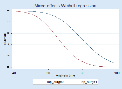
Survival analysis is widely used in medical research and social science to analyze the time until an event occurs (e.g., death, failure). Stata offers commands such as stset, stcox (for Cox regression), and streg (for parametric survival models) to perform survival analysis and estimate hazard rates.

Structural Equation Modeling (SEM)

SEM is a multivariate technique that allows researchers to examine complex relationships between variables. Stata has a built-in SEM package that allows for path analysis, confirmatory factor analysis, and latent variable modeling. The sem command in Stata makes it easy to specify and estimate models, providing tools for model diagnostics and comparison.

Bayesian Analysis

Bayesian methods are increasingly popular in various fields, especially when data is sparse or the prior information is crucial. Stata provides a Bayesian analysis suite, including bayesmh, bayesreg, and bayesprobit, among others. These tools allow users to perform Bayesian regression, estimation, and hypothesis testing with ease.

Machine Learning

With the release of Stata 16 and 17, Stata introduced various machine learning capabilities, allowing users to apply techniques such as random forests, LASSO regression, and k-means clustering. These methods are ideal for predictive modeling and can be implemented using commands like lasso and randomforest.

Advanced Statistical Analysis in Stata

Getting Stata

  • Stata Free Trial
    Stata offers a free trial version of its software, which allows users to test its capabilities before making a purchase. The trial version is often limited in terms of time (typically 30 days) and functionality but is a great way to explore the software.
  • Stata Price
    The price of Stata varies based on the version (IC, SE, MP) and the type of license (student, individual, or corporate). The basic version, Stata/IC, is suitable for most users, but those requiring advanced features, such as handling large datasets or parallel processing, can opt for Stata/SE or Stata/MP, which cost more.
  • Stata 17 Free Download
    Stata 17, the latest version of the software, is not available for free. However, users can download a free trial version from the official Stata website. This gives users an opportunity to explore the latest features and capabilities of Stata 17, including enhanced machine learning tools and support for bigger datasets.
  • Stata Full Meaning
    The name “Stata” is derived from the term “Statistics and Data.” It emphasizes its primary function as a tool for performing complex statistical analysis on large datasets.
  • Is Stata Free?
    No, Stata is not free. It requires a paid license for full use. The pricing is based on the type of user, with discounts for students and academic institutions. Stata also offers different licensing options depending on the number of users (single user or multiple users). However, the free trial version provides a short-term solution for those interested in testing the software.
  • Stata 18 Free Download
    Stata 18 has not been released yet, but it is expected to offer further enhancements to statistical analysis tools, machine learning, and data visualization capabilities. As with other versions, it is likely to offer a free trial upon its release, allowing users to test its new features.

Advanced Statistical Analysis in Stata

Conclusion

Stata is an excellent choice for advanced statistical analysis, offering a wide range of tools for complex data analysis across various fields. From multivariate regression to time series and machine learning, Stata provides the necessary resources to handle a broad spectrum of analytical challenges. While Stata is not free, it offers a free trial version for those who wish to explore its capabilities before purchasing. Researchers and analysts interested in advanced statistical techniques will find Stata to be a versatile and efficient tool in their toolkit.

Needs help with similar assignment?

We are available 24x7 to deliver the best services and assignment ready within 3-4 hours? Order a custom-written, plagiarism-free paper

Get Answer Over WhatsApp Order Paper Now

Stata Command Cheat Sheet for Beginners|2025

Stata Command Cheat Sheet for Beginners offers a quick reference guide to essential Stata commands. Learn key commands, functions, and tips to streamline your data analysis process and boost efficiency.

Stata is a widely-used software for data analysis, statistics, and econometrics. It provides a comprehensive set of tools for data manipulation, statistical analysis, and visualization. Whether you are working on social sciences, economics, or health data, mastering Stata commands is essential for effective data analysis. For beginners, a Stata command cheat sheet is an invaluable resource for learning and referencing essential commands. In this paper, we will explore some of the most frequently used Stata commands, organize them into categories, and provide an overview of useful resources like Stata command cheat sheets in PDF format or accessible online (GitHub).

Introduction to Stata

Stata is an integrated software package that allows users to manage, analyze, and graph data. Its user interface comprises the Command window, Results window, Variables window, and Review window. Stata also supports the use of Do-files for saving and executing a series of commands. The command syntax follows a clear and concise structure that enables users to carry out a wide variety of tasks, from simple data cleaning to advanced statistical analysis.

The Importance of a Stata Command Cheat Sheet

For beginners, understanding the vast range of Stata commands can be overwhelming. A cheat sheet can help users by providing quick references to the most common commands, saving time and effort when writing Stata scripts or conducting analyses. Whether you are performing basic data management tasks or executing advanced econometric models, a well-structured cheat sheet can be a key resource.

Stata commands are typically written in the Command window, and results are displayed in the Results window. By understanding the structure of these commands and their syntax, you can streamline your data analysis workflow. For those seeking to enhance their productivity, cheat sheets offer easy access to frequently used commands, saving both time and cognitive effort.

Stata Command Categories

Stata commands can be grouped into several categories based on their functionality. Below are some of the key categories:

  • Data Management
  • Data Exploration
  • Statistical Analysis
  • Graphics and Visualization
  • Econometrics

Stata Command Cheat Sheet for Beginners

Data Management

Data management in Stata involves tasks like importing data, cleaning datasets, and reshaping data. These commands are essential for preparing the dataset before analysis.

  • use: Loads a Stata dataset (.dta file) into memory.
    Syntax: use filename.dta
  • save: Saves the current dataset to a file.
    Syntax: save filename.dta
  • import: Imports data from a variety of formats (Excel, CSV, etc.).
    Syntax: import excel filename.xlsx, sheet("Sheet1") firstrow
  • describe: Provides a summary of the dataset’s structure.
    Syntax: describe
  • list: Lists data in the active dataset.
    Syntax: list varlist
  • drop: Removes variables or observations from the dataset.
    Syntax: drop varlist or drop if condition
  • rename: Renames variables in the dataset.
    Syntax: rename oldname newname
  • gen: Generates a new variable.
    Syntax: gen newvar = expression
  • replace: Replaces values in an existing variable.
    Syntax: replace varname = expression if condition
  • merge: Merges two datasets based on a common variable.
    Syntax: merge 1:1 varlist using dataset.dta

Data Exploration

Exploring your data is a crucial step in any analysis. These commands help you summarize, visualize, and check the quality of your data.

  • summarize: Provides descriptive statistics for variables in the dataset.
    Syntax: summarize varlist
  • tabulate: Creates frequency tables for categorical variables.
    Syntax: tabulate varname
  • correlate: Computes correlation coefficients between variables.
    Syntax: correlate varlist
  • histogram: Creates histograms for continuous variables.
    Syntax: histogram varname

Statistical Analysis

Once data exploration is complete, you can proceed with statistical analyses. Stata supports a wide array of statistical techniques ranging from basic descriptive statistics to advanced econometrics.

  • regress: Performs linear regression analysis.
    Syntax: regress dependent_var independent_vars
  • logit: Runs logistic regression for binary outcomes.
    Syntax: logit dependent_var independent_vars
  • anova: Performs analysis of variance (ANOVA).
    Syntax: anova dependent_var independent_var
  • ttest: Performs t-tests to compare means between two groups.
    Syntax: ttest varname, by(groupvar)
  • pwcorr: Computes pairwise correlations, with p-values.
    Syntax: pwcorr varlist, sig

Graphics and Visualization

Stata also provides powerful graphical capabilities for visualizing your data. Graphics commands help you display relationships between variables, distributions, and model results.

  • scatter: Creates scatter plots of two variables.
    Syntax: scatter yvar xvar
  • line: Creates line plots.
    Syntax: line yvar xvar
  • graph bar: Creates bar charts.
    Syntax: graph bar (mean) varname, over(groupvar)
  • histogram: Creates histograms.
    Syntax: histogram varname

Econometrics

For users in the field of econometrics, Stata offers commands tailored to advanced modeling and time-series analysis.

  • xtreg: Performs panel data regression (fixed and random effects).
    Syntax: xtreg dependent_var independent_vars, fe (for fixed effects)
  • ivregress: Performs instrumental variables regression.
    Syntax: ivregress 2sls dependent_var (endogenous_var = instrument_vars)
  • tsset: Declares a dataset as time-series data.
    Syntax: tsset timevar
  • arima: Fits an ARIMA model for time-series data.
    Syntax: arima varname, ar(1) ma(1)

Stata Command Cheat Sheet for Beginners

Stata Command Cheat Sheets and Resources

There are several resources available online to help beginners navigate Stata commands more effectively. Some of the most useful resources include downloadable PDFs, GitHub repositories, and interactive websites. Below are a few notable ones:

Stata Command Cheat Sheet for Beginners PDF

For many beginners, a PDF cheat sheet provides a compact and easy-to-reference guide to Stata commands. These cheat sheets typically contain the most essential commands organized by function, making it easier to look up specific commands when working in Stata. You can find several free downloadable PDFs online, including those created by Stata users, instructors, and other data analysts.

Stata Command Cheat Sheet for Beginners GitHub

GitHub is an excellent platform for accessing community-generated resources. Many users contribute their own cheat sheets, which often include Stata command lists, examples, and tips for usage. By searching GitHub for repositories related to “Stata command cheat sheet,” you can access various comprehensive resources. Some of these repositories also contain code snippets for common tasks, helping users get started quickly.

Stata 17 Command PDF

With each version of Stata, new features and commands are introduced. For users working with Stata 17, it is important to have a cheat sheet specific to the latest release. Many websites and forums provide downloadable PDFs that include the commands and features introduced in Stata 17, along with updates and enhancements to existing commands.

Stata Commands for Econometrics

Econometricians often rely on specific Stata commands for modeling and analysis. There are cheat sheets available that focus solely on commands used in econometrics, such as panel data regression, instrumental variables, and time-series analysis. These resources are invaluable for anyone conducting economic or policy analysis.

Stata Command Cheat Sheet for Beginners

Conclusion

Stata is a powerful tool for data analysis, and its extensive range of commands can be daunting for beginners. However, by utilizing a Stata command cheat sheet, beginners can quickly access the necessary commands and master their workflow in Stata. Whether you prefer PDF cheat sheets, GitHub repositories, or other resources, there are plenty of options to help streamline your Stata experience.

For those focused on econometrics or advanced statistical modeling, Stata offers a specialized set of tools that cater to these areas. As you become more proficient in Stata, you will likely develop a customized cheat sheet tailored to your specific needs. With time and practice, you will become more comfortable navigating Stata’s vast functionality and make the most of its powerful capabilities.

Needs help with similar assignment?

We are available 24x7 to deliver the best services and assignment ready within 3-4 hours? Order a custom-written, plagiarism-free paper

Get Answer Over WhatsApp Order Paper Now

How to Merge Datasets in Stata: A Comprehensive Guide|2025

How to Merge Datasets in Stata: A Comprehensive Guide provides detailed instructions on merging datasets efficiently in Stata. Learn the steps, commands, and best practices for seamless data integration.

Merging datasets is an essential task when working with data analysis and management. In Stata, merging allows you to combine datasets containing complementary information about the same units of observation. This paper provides a detailed guide to merging datasets in Stata, including various merging strategies, key commands, and best practices. Keywords such as merge Stata, merge m:1 Stata, Stata joinby vs merge, Stata merge different variable names, Many-to-many merge Stata, Stata merge if, Stata merge vs append, and Stata merge keep will be covered throughout this guide.

How to Merge Datasets in Stata

Understanding Merging in Stata

Merging in Stata refers to the process of combining two or more datasets based on one or more common variables, known as key variables. This process is central to data preparation, especially when the datasets contain different pieces of information about the same entities. Stata provides several methods to merge datasets depending on the structure of the data and the type of relationship between the datasets.

The basic syntax of Stata’s merge command is:

stata
merge 1:m varlist using filename

Here, 1:m specifies the type of merge, and varlist refers to the variables common to both datasets. The using filename part specifies the second dataset that is being merged into the dataset in memory.

Types of Merges in Stata

Stata supports different types of merges, depending on the relationship between the datasets. These include:

  1. One-to-One Merge (1:1): This type of merge is used when both datasets have a one-to-one correspondence for each observation. For instance, if each dataset contains one observation per individual (with unique IDs), a 1:1 merge is appropriate.
  2. One-to-Many Merge (1:m): This occurs when one dataset contains unique observations (e.g., each individual has only one record in the first dataset), while the other dataset has multiple records for each observation (e.g., repeated measurements for each individual). The 1:m type merge is used when one dataset contains a unique key variable, and the other contains duplicates for that key variable.
  3. Many-to-One Merge (m:1): This is the reverse of the one-to-many merge, where the first dataset contains multiple observations for each unit (e.g., multiple records per individual), and the second dataset has a unique key variable. The m:1 merge type combines the two datasets by matching on the key variable.
  4. Many-to-Many Merge (m:m): This type of merge is used when both datasets contain multiple records for the same unit. For example, if both datasets have repeated measurements or entries for each individual, the m:m merge combines the datasets by matching records where the key variables have matching values in both datasets.

Each of these merge types requires different commands and considerations. Stata’s merge syntax allows for precise control over the merging process, ensuring that the final dataset is constructed in a way that fits the analysis.

Merging Datasets with merge m:1 in Stata

The merge m:1 command is used when the first dataset contains many records for each observation (e.g., multiple entries per person), while the second dataset contains only one record per observation. This is a typical use case in panel data analysis or when an observation is recorded across multiple time points.

The syntax for a merge m:1 is:

stata
merge m:1 keyvariable using second_dataset

In this case, keyvariable is the common identifier (e.g., an individual ID), and the second_dataset contains one record for each individual.

Stata: joinby vs. merge

Stata offers both the merge and joinby commands to combine datasets. While the merge command is the most common tool for combining datasets based on key variables, the joinby command offers an alternative for certain situations.

  1. merge Command: The merge command is more restrictive and expects a defined relationship between the datasets, such as one-to-one, one-to-many, or many-to-one. It requires matching key variables to align the datasets.
  2. joinby Command: The joinby command is more flexible in that it performs a cross join, meaning it merges all combinations of observations from both datasets that share common values in one or more key variables. This is useful when datasets have many-to-many relationships, and you want to combine every matching record from both datasets.

For example, if both datasets contain repeated measures of the same units, joinby will match every possible pair of records with the same key variable value, whereas merge would require explicit one-to-one or many-to-one relationships.

How to Merge Datasets in Stata

Merging Datasets with Different Variable Names

In some cases, datasets may have the same type of information, but the variable names differ. Stata allows merging datasets with different variable names by renaming variables before or during the merge process.

Here’s a typical workflow for merging datasets with different variable names:

  1. Rename Variables: You can rename the variable in one dataset so it matches the other dataset’s variable name. For example:
    stata
    rename old_varname new_varname
  2. Merge with Renamed Variables: Once the variables are renamed, you can merge the datasets as usual:
    stata
    merge 1:m common_variable using dataset2

Alternatively, you can specify the using dataset’s variable names directly in the merge command, using the using() option.

Many-to-Many Merge in Stata

Many-to-many merges are more complex and can lead to larger and potentially confusing datasets. A many-to-many merge occurs when both datasets have multiple records for the same key variable, and you want to combine them.

In Stata, to perform a many-to-many merge, use the following syntax:

stata
merge m:m keyvariable using second_dataset

While merge m:m is available in Stata, it is often discouraged unless necessary. The results can become large and lead to duplicates that may not make sense depending on the context of your data.

Instead of a many-to-many merge, you may want to reconsider the structure of your datasets and try to transform them into a one-to-many or one-to-one structure, depending on the specific analysis.

Stata Merge with Conditional Statements (if)

Stata’s merge command allows for conditional merging using the if qualifier. This enables users to merge datasets based on certain conditions, such as merging only for specific observations that meet particular criteria.

For instance, to merge only observations where a certain condition is met, the following command could be used:

stata
merge 1:m keyvariable using dataset2 if age > 30

This command merges the datasets only for individuals aged over 30. The if qualifier is a powerful tool for filtering datasets before performing the merge.

Stata Merge vs. Append

While merging combines datasets based on common variables, appending stacks datasets on top of one another, adding observations without aligning variables.

  • Merge: Combines datasets by matching rows based on a key variable.
  • Append: Adds rows from one dataset to another, assuming that both datasets have the same variables.

Use merge when you need to align data based on shared variables and append when you simply need to add more rows of similar data.

For instance, appending datasets with the following command:

stata
append using dataset2

This command adds all observations from dataset2 to the dataset currently in memory.

How to Merge Datasets in Stata

Stata Merge Keep

When merging datasets, it’s essential to decide how to handle unmatched observations. The merge command allows users to keep or drop unmatched records using the keep() option.

The merge command has the following options to keep or drop observations:

  • keep(match): Keeps only the matched observations.
  • keep(keep) or keep(1): Keeps all observations in the primary dataset.
  • keep(using): Keeps all observations from the using dataset.

For example:

stata
merge 1:m keyvariable using dataset2, keep(match)

This will keep only the matched observations, excluding records that don’t have a corresponding match in the second dataset.

How to Merge Datasets in Stata

Conclusion

Merging datasets in Stata is a critical step in data preparation. Whether you are working with a one-to-one, one-to-many, or many-to-many relationship, understanding the merge command and the different options available is essential for combining datasets effectively.

Key considerations include selecting the appropriate type of merge (1:m, m:1, m:m), managing variable name differences, handling conditional merges with if, and using the keep() option to control which observations are retained. By mastering these techniques, users can efficiently combine datasets and ensure that their analyses are built on well-merged, organized data.

GetSPSSHelp is the best website for “How to Merge Datasets in Stata: A Comprehensive Guide” because it offers expert, step-by-step instructions for effectively merging datasets in Stata. The platform simplifies complex data integration tasks, providing clear explanations of the necessary commands and techniques. GetSPSSHelp also offers personalized support to ensure users can successfully merge datasets based on their specific needs. With affordable pricing and high-quality resources, it is an ideal choice for anyone looking to master Stata’s data management features. Additionally, 24/7 customer support ensures that help is always available, making GetSPSSHelp a trusted resource for merging datasets in Stata.

Needs help with similar assignment?

We are available 24x7 to deliver the best services and assignment ready within 3-4 hours? Order a custom-written, plagiarism-free paper

Get Answer Over WhatsApp Order Paper Now

How to Perform ANOVA in Stata|2025

How to Perform ANOVA in Stata provides a clear, step-by-step guide for conducting ANOVA analysis using Stata. Learn how to run tests, interpret results, and apply statistical techniques to your data.

Abstract

Analysis of Variance (ANOVA) is a powerful statistical technique used to analyze the differences between group means in a sample. It helps determine whether the differences in means across groups are statistically significant. This paper explains how to perform ANOVA using Stata, a statistical software package widely used in the social sciences, economics, and other research fields. It covers one-way ANOVA, two-way ANOVA, and repeated measures ANOVA, with explanations of the relevant Stata commands, step-by-step guides, and interpretation of results.


How to Perform ANOVA in Stata


Introduction to ANOVA

Analysis of Variance (ANOVA) is a statistical method used to compare the means of three or more groups to see if they are significantly different from each other. It is primarily used when the dependent variable is continuous, and the independent variable is categorical. ANOVA assesses whether the variation in the data can be attributed to the group differences or whether it is due to random chance. There are different types of ANOVA based on the structure of the independent variables:

  • One-way ANOVA: Used when there is one independent variable with multiple levels or categories.
  • Two-way ANOVA: Used when there are two independent variables, and the interaction between these variables is of interest.
  • Repeated Measures ANOVA: Used when the same subjects are measured multiple times.

In this paper, we will focus on how to perform these different types of ANOVA in Stata, using both commands and graphical methods for interpretation.


One-Way ANOVA in Stata

A One-way ANOVA is used to test the hypothesis that the means of different groups are equal. The groups are defined by one independent categorical variable. The basic assumptions of one-way ANOVA are:

  • The groups are independent of each other.
  • The dependent variable is continuous.
  • The residuals (errors) are normally distributed within each group.
  • The variances across the groups are equal (homogeneity of variance).

One-Way ANOVA Example in Stata

To perform a one-way ANOVA in Stata, you can use the anova command. Below is an example dataset, where we wish to examine if there are differences in test scores (dependent variable) across three teaching methods (independent variable).

stata
. anova test_score method

Here, test_score is the dependent variable, and method is the independent variable. Stata will return an F-statistic along with a p-value that allows you to assess the significance of the group differences.

Interpretation of Results

Stata outputs several components after running the ANOVA command:

  • F-statistic: This tests whether the means of the groups are different. The higher the F-statistic, the more likely the means differ.
  • P-value: This tells you whether the F-statistic is significant. A p-value less than 0.05 typically indicates that the means are significantly different.
  • Sum of squares: This shows the variation in the data explained by the model (between-group variation) and the residual variation (within-group variation).

If the p-value is less than 0.05, you reject the null hypothesis that the means are equal.


How to Perform ANOVA in Stata

Two-Way ANOVA in Stata

A Two-way ANOVA examines the effect of two independent variables on a dependent variable. It can also test if there is an interaction between the two independent variables, meaning that the effect of one variable depends on the level of the other variable.

Two-Way ANOVA Example in Stata

Suppose you want to examine how two factors—method and gender—affect test_score. The Stata command would be:

stata
. anova test_score method##gender

Here, method and gender are the independent variables, and the ## operator indicates that Stata should test both the main effects of method and gender, as well as their interaction effect.

Interpretation of Results

The output for two-way ANOVA will include:

  • Main effects: This shows whether method or gender significantly affects the dependent variable (test_score).
  • Interaction effect: This tells you whether the effect of one independent variable depends on the level of the other. If the interaction is significant, it suggests that the impact of one variable on the dependent variable changes depending on the other variable.

If the interaction is not significant, you can interpret the main effects independently. However, if the interaction is significant, you need to examine the interaction plots to understand the relationship more fully.


Repeated Measures ANOVA in Stata

A Repeated Measures ANOVA is used when the same subjects are measured multiple times, for example, when participants are tested under different conditions or over time. The key difference from standard ANOVA is that repeated measures violate the assumption of independence, as the observations are correlated.

Repeated Measures ANOVA Example in Stata

Suppose you have data where test scores are measured at three different time points (before, during, and after a treatment) for the same group of participants. The data would need to be in a long format, with one column for the participant identifier, one for the time point, and one for the test score.

To run a repeated measures ANOVA, use the anova command with the id variable and the repeated measure as follows:

stata
. anova test_score time_subject

Here, test_score is the dependent variable, time represents the different time points, and subject is the repeated measure variable.

Interpretation of Results

In repeated measures ANOVA, you are primarily interested in the within-subjects variation over time. Stata will output:

  • Main effect of time: This shows whether there is a significant change in the dependent variable over the repeated measurements.
  • Interaction effect: This indicates whether the effect of time on the dependent variable depends on the individual characteristics or some other factor.

If the p-value for the main effect of time is significant, it suggests that the test scores significantly differ over time.


How to Perform ANOVA in Stata

Advanced ANOVA: Two-Way Repeated Measures

In more complex designs, both the factors involved can be repeated measures. For example, in a study measuring test scores over time, both the participants and the time points can be considered repeated measures.

Two-Way Repeated Measures Example in Stata

For a design where both participants and time points are repeated measures, the command would look something like this:

stata
. anova test_score subject##time

Here, subject and time are both repeated measures, and ## signifies that you want Stata to assess both the main effects and the interaction effect.


Stata Commands for ANOVA

Here’s a summary of the key Stata commands for performing different types of ANOVA:

  • One-Way ANOVA:
    stata
    anova dependent_variable independent_variable
  • Two-Way ANOVA:
    stata
    anova dependent_variable independent_variable1##independent_variable2
  • Repeated Measures ANOVA:
    stata
    anova dependent_variable subject##time
  • Post-hoc Tests: After ANOVA, you may want to perform post-hoc tests to determine which specific group means differ. This can be done using the pwmean command:
    stata
    pwmean dependent_variable, over(group_variable)

How to Perform ANOVA in Stata

Visualizing ANOVA Results

Visualizing the results of an ANOVA is an essential part of interpreting the findings. Stata provides several ways to visualize the results, including interaction plots, box plots, and means plots.

For instance, to plot the means of different groups in a one-way ANOVA, you can use the graph command:

stata
. graph box dependent_variable, over(group_variable)

For two-way ANOVA, interaction plots can be created using:

stata
. interactionplot dependent_variable, by(independent_variable1) by(independent_variable2)

These plots help visually inspect how the dependent variable changes across levels of the independent variables.


How to Interpret ANOVA Results in Stata

When interpreting the results of ANOVA in Stata, you must focus on:

  • F-statistic: It compares the variance between groups to the variance within groups. A higher F-statistic indicates that the group means differ more significantly.
  • P-value: The p-value tells you whether the observed differences are statistically significant. A p-value less than 0.05 suggests that the differences in means are unlikely to have occurred by chance.
  • Post-hoc Tests: If the overall ANOVA is significant, post-hoc tests can help identify which groups differ from each other.
  • Interaction Effects: If you are conducting a two-way ANOVA, pay attention to whether the interaction between the two independent variables is significant, as this indicates the presence of joint effects.

How to Perform ANOVA in Stata

Conclusion

ANOVA is an essential statistical tool for comparing means across multiple groups, and Stata provides an efficient way to perform and interpret this analysis. Whether you are conducting one-way ANOVA, two-way ANOVA, or repeated measures ANOVA, Stata’s robust commands allow you to easily execute the tests and understand the results. By carefully interpreting the F-statistic, p-value, and post-hoc tests, researchers can draw valid conclusions about the factors influencing their dependent variables.

As with any statistical method, the key to success with ANOVA lies in understanding the assumptions, checking the validity of those assumptions, and correctly interpreting the results. With these insights, Stata can be an invaluable tool for anyone conducting ANOVA in their research.

Needs help with similar assignment?

We are available 24x7 to deliver the best services and assignment ready within 3-4 hours? Order a custom-written, plagiarism-free paper

Get Answer Over WhatsApp Order Paper Now

Stata Assignment Help for Students: A Comprehensive Guide|2025

Stata Assignment Help for Students offers expert assistance with Stata projects and homework. Get personalized guidance, accurate solutions, and timely support to excel in your academic data analysis tasks.

Stata is a powerful statistical software used widely in various fields, particularly in economics, social sciences, health research, and data analysis. Many students across different disciplines rely on Stata to conduct statistical analyses, manage data, and interpret results. However, mastering Stata can be a challenge due to its complex commands, intricate functions, and various capabilities. This paper provides a detailed guide on Stata assignment help for students, highlighting common difficulties, offering solutions, and exploring resources that can assist students in mastering Stata for academic success.

Stata Assignment Help for Students

What is Stata?

Stata is a comprehensive software package designed for data analysis, data management, and graphics. It is widely used by professionals in academia and research fields for statistical analysis, particularly in economics, political science, sociology, biostatistics, and other quantitative disciplines. Stata offers a range of features including data manipulation, statistical modeling, graphical representations, and automated reports. Its strength lies in its user-friendly interface, powerful command syntax, and extensive support for statistical methods, making it a top choice for researchers.

Common Issues Students Face in Stata Assignments

While Stata is an excellent tool for data analysis, students often encounter several difficulties when working on assignments. Some of the most common issues include:

Understanding Stata Syntax

Stata’s syntax, although intuitive for some, can be overwhelming for beginners. The software operates through a command-based interface, where users must input specific commands to perform tasks. Many students struggle to learn the proper syntax and to interpret the results. Incorrect syntax can lead to errors or inaccurate results, which can affect the quality of assignments.

Data Import and Cleaning

Data cleaning is one of the most critical steps in data analysis, and it can be challenging for students new to Stata. Importing datasets from different file formats such as CSV, Excel, or SPSS into Stata may cause issues related to variable types, missing data, or incorrect variable labeling. Students often face difficulties in cleaning data, handling missing values, and transforming variables appropriately for analysis.

Performing Statistical Analysis

Stata provides a broad array of statistical tools such as regression analysis, ANOVA, time-series analysis, and hypothesis testing. However, selecting the right statistical method, applying the correct commands, and interpreting results can be confusing for students. Many students require help in understanding the intricacies of various statistical techniques and ensuring they are applied correctly in their assignments.

Working with Large Datasets

Stata can handle large datasets, but when working with substantial volumes of data, students may encounter performance issues or face difficulties in managing the data efficiently. Optimizing memory usage and ensuring smooth processing for large datasets can be a complex task.

Graphing and Visualization

Creating graphs and visualizations in Stata can be a daunting task for students, especially when they are unfamiliar with the different types of graphs available (e.g., scatter plots, bar charts, histograms). Students often need help with formatting graphs and customizing them for better presentation and clarity.

Debugging Errors

Stata can produce error messages that may confuse students, especially beginners. Understanding error messages and resolving coding mistakes can be one of the biggest hurdles when working with Stata for assignments.

Stata Assignment Help for Students

How to Overcome Challenges in Stata Assignments

To tackle these challenges effectively, students can adopt the following strategies:

Learn Basic Stata Commands

To work efficiently in Stata, students should familiarize themselves with the most commonly used commands. Some essential commands include:

  • use: to load a dataset.
  • describe: to get an overview of the data.
  • summarize: to compute descriptive statistics.
  • regress: to perform regression analysis.
  • tabulate: to create frequency tables.
  • generate: to create new variables.

Understanding these basic commands can help students navigate Stata effectively and avoid common errors in their assignments.

Practice Data Importing and Cleaning

Data cleaning is a critical aspect of any analysis. Students should practice importing different file formats into Stata and learn how to handle data inconsistencies, missing values, and data transformations. Stata provides various tools such as insheet, import excel, and merge to import and manipulate data. Additionally, students should explore the egen command to generate new variables or aggregate data.

Seek Guidance from Online Resources

One of the most effective ways to overcome the difficulties of working with Stata is by utilizing online resources. Many websites, forums, and YouTube channels offer free tutorials, guides, and step-by-step instructions on using Stata. Some popular online platforms include:

  • Stata’s Official Website: The official documentation and tutorials provided by Stata are invaluable for learning the software.
  • Statalist: A community forum where users discuss common issues and share solutions to Stata-related problems.
  • YouTube: Channels like “StataCorp” and “Data Science Dojo” offer video tutorials on a range of Stata topics.
  • Coursera and Udemy: These platforms offer courses dedicated to mastering Stata and using it for statistical analysis.

Consult Stata Assignment Help Services

For students who need additional assistance with their Stata assignments, many professional assignment help services are available. These services provide expert support on Stata-related tasks, including data analysis, model building, and report generation. Students can benefit from:

  • Expert Stata Tutors: Many online platforms offer one-on-one tutoring with experts in Stata, where students can ask questions and get personalized help.
  • Stata Assignment Writing Services: These services help students complete their Stata assignments by writing reports, performing data analysis, and offering clear interpretations of results.
  • Sample Assignments: Some websites provide sample Stata assignments to help students understand how to approach problems and present solutions effectively.

Practice Regularly

The key to mastering Stata is consistent practice. By working through various datasets and assignments, students can become more comfortable with the software’s commands and functions. Practicing with real-life datasets can help students understand the practical applications of Stata and develop their analytical skills.

Debugging and Error Resolution

If students encounter errors in Stata, they should carefully examine the error message to identify the issue. Common errors may include misspelled commands, incorrect variable names, or missing data. Students should also refer to the Stata Help feature, which provides information on various commands and error types. Debugging through trial and error and using the Stata community forums can also help students resolve issues effectively.

Stata Assignment Help for Students

Benefits of Stata Assignment Help Services

For students struggling with Stata assignments, seeking professional help can offer several benefits:

Time-Saving

Stata assignments can be time-consuming, especially for students who are unfamiliar with the software. Professional Stata assignment help services can assist students in completing their assignments efficiently, allowing them to focus on other academic tasks.

Expert Guidance

Experienced Stata tutors or assignment help providers can offer expert guidance and ensure that students use the correct methodology, interpret results accurately, and meet assignment requirements.

Improved Academic Performance

By receiving personalized help and learning from expert solutions, students can improve the quality of their assignments and gain a deeper understanding of Stata. This leads to better grades and a stronger grasp of statistical analysis.

Customized Solutions

Assignment help services provide customized solutions tailored to each student’s needs. Whether students require help with data analysis, writing reports, or creating graphs, these services can provide step-by-step assistance.

Learning Resources

Stata assignment help services often provide valuable learning resources such as tutorials, sample codes, and practice exercises. These resources can further enhance students’ understanding of Stata and statistical analysis.

Stata Assignment Help for Students

Conclusion

Stata is a powerful tool for students pursuing degrees in disciplines that require data analysis, but it can be challenging to learn and use effectively. Common difficulties such as mastering syntax, cleaning data, performing statistical analysis, and debugging errors often lead students to seek help. By familiarizing themselves with the software, practicing regularly, and utilizing online resources and professional help, students can overcome these challenges and succeed in their Stata assignments. Whether it is through self-study, tutoring, or assignment help services, there are numerous ways for students to improve their Stata skills and achieve academic success.

Needs help with similar assignment?

We are available 24x7 to deliver the best services and assignment ready within 3-4 hours? Order a custom-written, plagiarism-free paper

Get Answer Over WhatsApp Order Paper Now