How to Do Regression Analysis in Stata|2025
How to Do Regression Analysis in Stata offers a step-by-step guide to performing regression analysis using Stata. Learn essential techniques for interpreting results and applying them to your data.
Regression analysis is a fundamental statistical method for exploring relationships between variables and making predictions. Stata, a widely-used statistical software, offers robust tools to perform various regression analyses, from simple linear regression to more complex logistic regression. This guide provides a comprehensive overview of how to perform regression analysis in Stata and interpret the results effectively.
Introduction to Regression Analysis in Stata
Regression analysis is a statistical method used to model and analyze relationships between a dependent variable (outcome) and one or more independent variables (predictors). Stata simplifies this process through its user-friendly commands and intuitive output.
This document covers the following topics:
- Performing linear regression in Stata
- Interpreting Stata regression output
- Performing multiple linear regression
- Conducting logistic regression
- Creating and interpreting regression output tables
Setting Up Data for Regression Analysis
Before performing any regression analysis, it’s essential to ensure that your data is clean and properly formatted. In Stata:
- Load your dataset:
use "dataset.dta", clear - Check for missing values:
misstable summarize - Examine the variables:
describe
summarize
Linear Regression in Stata

Command for Linear Regression
Linear regression models the relationship between a dependent variable and one or more independent variables. In Stata, the primary command for linear regression is:
regress dependent_variable independent_variablesFor example:
regress y x1 x2 x3This command specifies y as the dependent variable and x1, x2, and x3 as the independent variables.
Interpreting Stata Regression Output
After running the regression command, Stata produces a detailed output table. Key components include:
- Coefficients: These indicate the change in the dependent variable for a one-unit change in the independent variable.
- Standard Errors: Measure the variability of the coefficient estimates.
- t-Statistics and p-Values: Indicate whether the coefficients are statistically significant.
- R-squared: Shows the proportion of variance in the dependent variable explained by the independent variables.
Example Output
      Source |       SS           df       MS              Number of obs =     100
-------------+----------------------------------           F(  3,   96) =    15.45
       Model |   123.4567         3   41.15223             Prob > F      =    0.0000
    Residual |   456.7890        96   4.75510             R-squared     =    0.2123
-------------+----------------------------------           Adj R-squared =    0.1832
       Total |   580.2457        99   5.85905             Root MSE      =    2.1819

------------------------------------------------------------------------------
          y |      Coef.   Std. Err.      t    P>|t|     [95% Conf. Interval]
-------------+----------------------------------------------------------------
         x1 |   1.234567   0.456789     2.70   0.008      0.324567    2.145678
         x2 |  -0.345678   0.123456    -2.80   0.006     -0.590123   -0.101234
         x3 |   0.567890   0.078901     7.19   0.000      0.411123    0.724567
       _cons |   2.345678   1.234567     1.90   0.061     -0.097890    4.789123
------------------------------------------------------------------------------
Key Takeaways
- Significance: Look at the p-values. If
P>|t|is less than 0.05, the variable significantly predicts the dependent variable. - Effect Size: Examine the coefficients. For instance, a coefficient of
1.234567forx1means a one-unit increase inx1increasesyby approximately 1.23 units. - Model Fit: Check R-squared and adjusted R-squared to assess how well the model explains the variance in
y.
Multiple Linear Regression in Stata
Multiple linear regression involves two or more independent variables. The command is the same as for simple regression:
regress dependent_variable independent_variablesFor instance:
regress income education experience ageInterpretation
In multiple regression, each coefficient represents the effect of the corresponding independent variable while controlling for the others. Ensure multicollinearity is not a problem by checking the Variance Inflation Factor (VIF):
vifIf VIF values are above 10, consider removing or combining variables.
Logistic Regression in Stata
Logistic regression models a binary outcome variable (e.g., success/failure). Use the logit or logistic commands:
logit dependent_variable independent_variablesExample:
logit disease age bmi smokingInterpreting Logistic Regression Output
Logistic regression output differs slightly from linear regression:
- Coefficients (Log Odds): Represent the change in the log odds of the dependent variable for a one-unit change in the predictor.
- Odds Ratios: Use the
oroption to display odds ratios instead of log odds:logit disease age bmi smoking, or - Significance: Like linear regression, check the p-values.
Example Output
Logistic regression                               Number of obs     =     500
                                                  LR chi2(3)        =   45.89
                                                  Prob > chi2       =   0.0000
Log likelihood = -300.45678                       Pseudo R2         =   0.0712

------------------------------------------------------------------------------
     disease | Odds Ratio   Std. Err.      z    P>|z|     [95% Conf. Interval]
-------------+----------------------------------------------------------------
         age |   1.045678   0.012345     3.70   0.000      1.021234    1.070123
         bmi |   1.234567   0.067890     4.56   0.000      1.103456    1.381234
     smoking |   2.567890   0.345678     7.43   0.000      1.890123    3.456789
------------------------------------------------------------------------------
Key Takeaways
- Odds Ratios: An odds ratio greater than 1 indicates increased odds of the outcome; less than 1 indicates decreased odds.
- Significance: Look at the p-values for each variable.
- Model Fit: Use the likelihood ratio chi-square and pseudo R-squared values.
Creating and Interpreting Stata Regression Output Tables
Stata makes it easy to export regression results into professional tables using commands like outreg2 or esttab.
Exporting Results with outreg2
- Install the command:
ssc install outreg2 - Save results to a Word or Excel file:
outreg2 using results.doc, replace word - To include multiple models:
eststo model1: regress y x1 x2
eststo model2: regress y x1 x2 x3
esttab model1 model2 using results.doc, replace
Interpretation of Stata Output PDF
Once the results are exported, you can create PDFs for distribution. Pay close attention to:
- Consistency: Ensure all relevant statistics (coefficients, p-values, confidence intervals) are included.
- Clarity: Use clear labels for variables and models.
Tips for Effective Regression Analysis in Stata
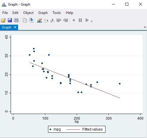
- Visualize Relationships: Use scatterplots and histograms before modeling:
scatter y x histogram x - Check Assumptions: Ensure the assumptions of regression (e.g., linearity, homoscedasticity) are met:
estat hettest - Model Diagnostics: Evaluate the model using residual plots:
rvfplot

Conclusion
Regression analysis in Stata is a powerful method for uncovering relationships in data. By understanding the commands, interpreting the output, and utilizing tools like outreg2, you can perform robust analyses and present your findings effectively. This guide provides a solid foundation, but continual practice and exploration of Stata’s capabilities will enhance your proficiency.
Needs help with similar assignment?
We are available 24x7 to deliver the best services and assignment ready within 3-4 hours? Order a custom-written, plagiarism-free paper