How to Perform Multiple Linear Regression in R: A Step-by-Step Guide|2025
Learn How to Perform Multiple Linear Regression in R with step-by-step guidance. Discover key functions, interpretation, and best practices for accurate analysis.
Multiple linear regression is a statistical technique used to model the relationship between a dependent variable and two or more independent variables. The goal is to predict the value of the dependent variable based on the values of the independent variables. In R, performing multiple linear regression is straightforward and involves using a variety of packages and functions to analyze data. This paper walks through the process of performing multiple linear regression in R, including understanding the syntax, interpreting results, handling categorical variables, and visualizing the model.
Introduction to Multiple Linear Regression
Multiple linear regression is an extension of simple linear regression, where the dependent variable is modeled as a linear combination of multiple independent variables. This technique is widely used in fields like economics, healthcare, and social sciences to understand how different factors affect a particular outcome.
In the context of R, multiple linear regression can be performed easily using the lm() function, which stands for “linear model.” The general formula for multiple linear regression is as follows:
Y=β0+β1X1+β2X2+⋯+βnXn+ϵY = \beta_0 + \beta_1 X_1 + \beta_2 X_2 + \dots + \beta_n X_n + \epsilon
Where:
- YY is the dependent variable
- β0\beta_0 is the intercept
- β1,β2,…,βn\beta_1, \beta_2, \dots, \beta_n are the coefficients of the independent variables X1,X2,…,XnX_1, X_2, \dots, X_n
- ϵ\epsilon is the error term
How to Perform Multiple Linear Regression in R Step-by-Step
Step 1: Install and Load Necessary Packages
Before performing multiple linear regression, make sure that you have installed the necessary packages. Although the lm() function is part of base R, additional packages such as ggplot2 for visualization can be useful. To install these packages, use the following commands:
Step 2: Load the Data
The next step is to load your dataset into R. For this example, we will use a built-in dataset called mtcars, which contains data about different car models, including variables like miles per gallon (mpg), horsepower, and weight. You can load your own dataset by using the read.csv() function.
Step 3: Inspect the Data
Before proceeding, it is crucial to inspect the data to understand its structure. Use functions like head(), summary(), and str() to take a quick look at the data.
Step 4: Fit the Multiple Linear Regression Model
Now that you have your data, you can fit the multiple linear regression model using the lm() function. In this example, we want to predict the miles per gallon (mpg) based on the other variables in the dataset.
In this command:
mpgis the dependent variablewt,hp,qsec, anddratare the independent variablesdata = mtcarsspecifies that the data is in themtcarsdataset
Step 5: View the Summary of the Model
Once the model is fitted, you can view a summary of the regression results by using the summary() function. This will show important statistics like the coefficients, p-values, R-squared, and adjusted R-squared.
The output will display the coefficients for each independent variable, as well as the statistical significance of these variables in predicting mpg.
How to Perform Multiple Linear Regression in R Using the lm() Function
The lm() function in R is a flexible way to perform multiple linear regression. The syntax for this function is as follows:
formula: A symbolic description of the model (e.g.,mpg ~ wt + hp)data: The dataset containing the variables
In the previous example, the formula mpg ~ wt + hp + qsec + drat is used to predict mpg based on four predictors. The function will return a linear model object that contains the fitted regression coefficients and other important statistics.
Multiple Linear Regression in R with ggplot2
Visualizing the results of multiple linear regression can help understand the relationships between variables. ggplot2 is a powerful visualization package in R that can be used to create a range of plots, including those to visualize regression models.
Step 1: Basic Scatter Plot
A simple scatter plot can be created to visualize the relationship between the dependent and independent variables. For instance, to plot mpg against wt, use:
In this plot:
aes(x = wt, y = mpg)defines the axesgeom_point()adds the scatter pointsgeom_smooth(method = "lm")adds the regression line
Step 2: Multiple Regression Plot
When dealing with multiple predictors, it can be challenging to visualize the relationship directly. However, you can create pair plots for a subset of variables to see how they relate to each other.
This will generate a matrix of scatter plots, showing pairwise relationships between the selected variables.
How to Plot Multiple Linear Regression in R
To visualize a multiple linear regression model with more than one independent variable, you can plot residuals or use diagnostic plots. The plot() function in R allows you to generate residual plots, leverage plots, and Q-Q plots to evaluate the model’s fit.
This will display:
- A residuals vs. fitted values plot
- A normal Q-Q plot for the residuals
- A scale-location plot
- A Cook’s distance plot
These plots help identify problems like heteroscedasticity, non-normality, or influential data points.
Interpreting Multiple Linear Regression Results in R
Interpreting the results of a multiple linear regression involves understanding the coefficients, p-values, R-squared value, and residuals.
Coefficients
The coefficients represent the change in the dependent variable for a one-unit change in the independent variable. For example, if the coefficient for wt is -3.1, it means that for every unit increase in the weight of a car, the mpg decreases by 3.1 units.
P-values
The p-value tests the null hypothesis that a particular coefficient is zero. If the p-value is less than 0.05, you can reject the null hypothesis and conclude that the variable has a significant effect on the dependent variable.
R-squared
The R-squared value represents the proportion of the variance in the dependent variable that is explained by the independent variables. A higher R-squared value indicates a better fit of the model to the data.
Multiple Linear Regression in R with Categorical Variables
Multiple linear regression in R can also handle categorical variables by converting them into dummy variables. This is done automatically when you include factors in the model.
For example, if the mtcars dataset contained a categorical variable like cyl (number of cylinders), you could include it in the regression model as follows:
R will automatically create dummy variables for cyl (e.g., cyl4, cyl6, cyl8) and include them in the model.
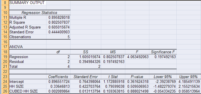
Example: Performing Multiple Linear Regression in Excel
Although R is a powerful tool for performing multiple linear regression, you can also perform regression analysis in Excel. Excel offers a built-in regression tool under the Data Analysis package.
To perform multiple linear regression in Excel:
- Organize your data in columns, with the dependent variable in one column and the independent variables in the other columns.
- Open the Data Analysis Toolpak by selecting
Data>Data Analysis>Regression. - Select your input range for the dependent and independent variables.
- Click
OKto run the regression analysis.
Excel will provide you with a summary output similar to R, including coefficients, R-squared, p-values, and other statistics.
Conclusion
Multiple linear regression is a fundamental statistical method that allows you to model relationships between variables and make predictions. R provides a powerful and flexible environment for performing multiple linear regression, visualizing the results, and interpreting the findings. By following the steps outlined in this paper, you can easily perform multiple linear regression in R and gain valuable insights into your data.
For more advanced analyses, you can experiment with additional techniques like regularization (e.g., Lasso and Ridge regression), interaction terms, and polynomial regression. Whether you’re working with continuous or categorical variables, R’s capabilities make it an ideal tool for performing complex regression analyses.
Needs help with similar assignment?
We are available 24x7 to deliver the best services and assignment ready within 3-4 hours? Order a custom-written, plagiarism-free paper


