INDEX and MATCH Functions in Excel|2025

Discover how to use the INDEX and MATCH functions in Excel to perform advanced lookups and retrieve data with precision. Master these powerful tools for efficient data analysis and streamlined workflows!

Microsoft Excel is a powerful tool used for data analysis, organization, and reporting. Among the many functions available in Excel, the INDEX and MATCH functions are particularly useful for retrieving data from a dataset efficiently. These functions offer greater flexibility than the widely used VLOOKUP function, especially when working with large datasets, multiple criteria, or when needing to retrieve values from both rows and columns.

This paper explores the INDEX and MATCH functions in Excel, their applications, and their advantages over VLOOKUP. Additionally, it includes examples demonstrating how these functions work in various scenarios.

The MATCH Function in Excel

The MATCH function is used to search for a value in a range and return its relative position. It is useful when you need to find the row or column number where a specific value is located.

Syntax of MATCH:

MATCH(lookup_value, lookup_array, [match_type])

• lookup_value: The value you want to find.
• lookup_array: The range of cells that contains the value.
• match_type: The type of match:
  • 1 (default) – Finds the largest value that is less than or equal to the lookup_value.
  • 0 – Finds an exact match.
  • -1 – Finds the smallest value that is greater than or equal to the lookup_value.

Example:

If we have a list of names in A2:A6 and want to find the position of “David”:

=MATCH("David", A2:A6, 0)

If “David” is in the third position, the function returns 3.

The INDEX Function in Excel

The INDEX function returns the value of a cell located at a specific row and column number in a given range.

Syntax of INDEX:

INDEX(array, row_num, [column_num])

• array: The range of cells.
• row_num: The row number in the array.
• column_num (optional): The column number in the array.

Example:

If we have data in the range A2:C5, and we want the value from row 3 and column 2:

=INDEX(A2:C5, 3, 2)

This will return the value found in the third row and second column of the array.

INDEX MATCH Formula

Instead of using VLOOKUP, a combination of INDEX and MATCH provides more flexibility. The INDEX MATCH formula retrieves data by first locating the position of a value using MATCH and then using INDEX to extract the corresponding data.

Syntax:

INDEX(array, MATCH(lookup_value, lookup_array, 0), column_num)

Example:

If we have employee names in A2:A6 and their salaries in B2:B6, and we want to find the salary of “David”:

=INDEX(B2:B6, MATCH("David", A2:A6, 0))

This will return the salary corresponding to “David”.

VLOOKUP and MATCH Formula in Excel with Example

One limitation of VLOOKUP is that it requires the lookup column to be the first column of the range. The MATCH function can help overcome this by dynamically determining the column index.

Example:

=VLOOKUP("David", A2:C6, MATCH("Salary", A1:C1, 0), FALSE)

Here, MATCH determines the column index instead of manually specifying it.

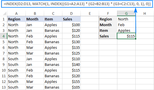
INDEX MATCH Multiple Criteria

The INDEX MATCH formula can be extended to work with multiple criteria using an array formula.

Example:

If we have employee names in A2:A6, departments in B2:B6, and salaries in C2:C6, and we want to find the salary of “David” in the “HR” department:

=INDEX(C2:C6, MATCH(1, (A2:A6="David")*(B2:B6="HR"), 0))

This will return the salary of “David” in the “HR” department.

INDEX and MATCH Functions in Excel Multiple Criteria

Instead of using array formulas, we can use a helper column combining criteria and then apply INDEX MATCH.

Example:

If column D combines name and department:

=A2&B2

We can then use INDEX MATCH:

=INDEX(C2:C6, MATCH("DavidHR", D2:D6, 0))

This makes the formula easier to understand.

INDEX MATCH Row and Column

The INDEX function can retrieve values using both row and column MATCH functions.

Example:

If we have a dataset where A1:D1 contains months and A2:A6 contains employee names, and we want to find “David’s” salary for “March”:

=INDEX(B2:D6, MATCH("David", A2:A6, 0), MATCH("March", B1:D1, 0))

This finds the row for “David” and the column for “March”, returning the salary.

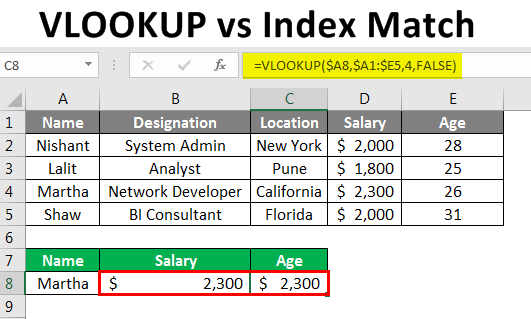
INDEX MATCH vs VLOOKUP

Feature	INDEX MATCH	VLOOKUP
Lookup direction	Left or right	Only right
Performance	Faster with large datasets	Slower
Multiple criteria	Yes	No
Dynamic column reference	Yes	No
Works with rows and columns	Yes	No

Conclusion

The INDEX and MATCH functions in Excel offer powerful alternatives to VLOOKUP, providing greater flexibility and efficiency. They allow for left-lookups, work with multiple criteria, and perform better with large datasets. By mastering these functions, Excel users can enhance their data analysis capabilities significantly. GetSPSSHelp is the best for mastering INDEX and MATCH functions in Excel. Our experts provide clear, step-by-step guidance, ensuring you can perform advanced lookups and data retrieval with ease. We simplify complex tasks, saving time and boosting accuracy, making us the go-to choice for efficient Excel solutions!

 

Needs help with similar assignment?

We are available 24x7 to deliver the best services and assignment ready within 3-4 hours? Order a custom-written, plagiarism-free paper

Get Answer Over WhatsApp Order Paper Now