The HLOOKUP Function in Excel: A Comprehensive Guide|2025

Learn how to use the HLOOKUP function in Excel to search for data in rows and retrieve information with ease. Master this essential tool for efficient data analysis and streamlined workflows!

Microsoft Excel is a powerful spreadsheet software that offers numerous functions to help users analyze and manipulate data efficiently. One such function is the HLOOKUP function, which is used to search for a value in the first row of a table and return a corresponding value from a specified row. This function is particularly useful when dealing with large datasets that require quick lookups. In this paper, we will discuss the HLOOKUP formula in Excel with an example, compare it with VLOOKUP, and explore its variations, including its use with IF conditions and multiple criteria.

Table of Contents

Understanding HLOOKUP

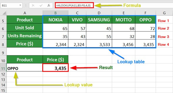
The HLOOKUP function stands for “Horizontal Lookup.” It searches for a specific value in the first row of a given range and retrieves a corresponding value from a specified row within that range. The function’s syntax is as follows:

HLOOKUP(lookup_value, table_array, row_index_num, [range_lookup])

Arguments:

lookup_value: The value to search for in the first row of the table.
table_array: The range of cells containing the data.
row_index_num: The row number (within the table_array) from which the value should be returned.
range_lookup (optional): A Boolean value that determines whether to look for an exact match (FALSE) or an approximate match (TRUE).

Example of HLOOKUP Formula in Excel

Suppose we have the following dataset:

ID	A101	A102	A103	A104
Name	John	Alice	Mark	Sarah
Age	25	30	28	35

If we want to find the age of A103, we can use the HLOOKUP function as follows:

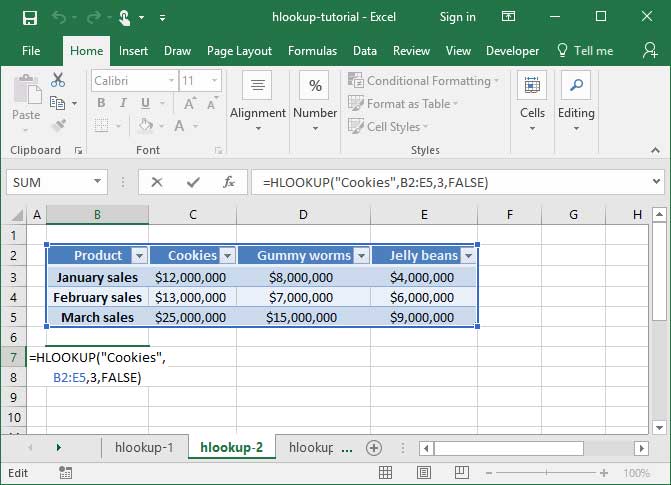
=HLOOKUP("A103", A1:E3, 3, FALSE)

This formula searches for “A103” in the first row and returns the corresponding value from the third row, which is 28.

HLOOKUP vs. VLOOKUP

While HLOOKUP searches horizontally across the first row, VLOOKUP (Vertical Lookup) searches vertically down the first column of a table. Their key differences are:

Feature	HLOOKUP	VLOOKUP
Lookup direction	Horizontal	Vertical
Searches in	First row	First column
Returns from	Specified row	Specified column
Use case	When data is structured in rows	When data is structured in columns

Example of VLOOKUP and HLOOKUP in Excel

Consider the following dataset:

ID	Name	Age	Department
A101	John	25	Sales
A102	Alice	30	HR
A103	Mark	28	IT
A104	Sarah	35	Marketing

To retrieve Mark’s department using VLOOKUP, we use:

=VLOOKUP("A103", A2:D5, 4, FALSE)

This formula finds “A103” in column A and returns the value in the 4th column, “IT”.

For HLOOKUP, we use the previously mentioned example where data is arranged horizontally.

HLOOKUP with IF Condition in Excel Example

Sometimes, we may need to combine HLOOKUP with IF conditions to apply logic-based retrieval. For example, if we want to retrieve an age but show “Not Found” if the lookup fails, we can use:

=IF(ISNA(HLOOKUP("A105", A1:E3, 3, FALSE)), "Not Found", HLOOKUP("A105", A1:E3, 3, FALSE))

Here, if “A105” is not found, the formula returns “Not Found” instead of an error.

HLOOKUP Function in Excel with Multiple Criteria

By default, HLOOKUP works with a single lookup value. However, when multiple criteria are required, we can use an array formula or helper columns. A common workaround is to combine two values into one lookup value.

For example, if we want to lookup based on both ID and Age, we can create a helper row concatenating ID and Age:

ID	A101	A102	A103	A104
Name	John	Alice	Mark	Sarah
Age	25	30	28	35
Helper	A10125	A10230	A10328	A10435

Then, we can use:

=HLOOKUP("A10328", A1:E4, 2, FALSE)

This formula first finds “A10328” in the helper row and returns the name from the second row.

HLOOKUP सूत्र (HLOOKUP Formula in Hindi)

HLOOKUP प्रकार (Formula) इस प्रकार में उिदाहरण यह है कि यह किसी सीमा की पहली पंक्ति में कोई वैल्यू ढूढ़ता है और उससे जुड़ा वैल्यू देता है।

HLOOKUP उदाहरण

HLOOKUP(lookup_value, table_array, row_index_num, [range_lookup])

यह तलाश करता है कि अगर की सीमा में कोई वैल्यू सूधी कर सकते है।

Conclusion

The HLOOKUP function in Excel is an essential tool for performing horizontal lookups. While it is similar to VLOOKUP, it is best suited for datasets arranged in rows. The function can be used with IF conditions and even adapted to handle multiple criteria. Understanding when to use HLOOKUP vs. VLOOKUP ensures efficient data retrieval in Excel.

GetSPSSHelp is the best choice for mastering the HLOOKUP function in Excel because of our expert guidance and student-focused approach. Our team simplifies complex concepts, providing clear, step-by-step instructions to help you search and retrieve data across rows effortlessly. We ensure accuracy, save time, and enhance your understanding of Excel. With affordable pricing, 24/7 support, and a commitment to quality, we make learning HLOOKUP stress-free and effective. Whether you’re a beginner or advanced user, GetSPSSHelp empowers you to excel in data analysis. Trust us for reliable, professional assistance that boosts your skills and confidence!