The SUMIF and SUMIFS Functions in Excel: A Comprehensive Guide|2025
/in Advanced Excel Articles /by BesttutorDiscover how to use the SUMIF and SUMIFS functions in Excel to sum data based on single or multiple conditions. Master these powerful tools for efficient data analysis and reporting!
Excel has become a powerful tool for data analysis and manipulation, offering a vast range of functions to help users perform complex tasks. Among these functions, the SUMIF and SUMIFS functions stand out as essential tools for summing values based on specified conditions. Both functions provide an efficient way to sum data based on criteria, making them indispensable for analyzing large datasets. This paper aims to explore these functions in depth, comparing their capabilities and offering practical examples of their usage.
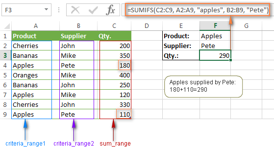
Table of Contents
ToggleOverview of SUMIF and SUMIFS Functions
Both the SUMIF and SUMIFS functions in Excel are used to sum values in a range based on certain criteria. However, they differ in terms of the number of conditions (criteria) they can handle.
SUMIF Function in Excel
The SUMIF function is used to sum values in a range based on a single condition or criteria. It is ideal for simple data analysis tasks where you only need to apply one condition. The syntax of the SUMIF function is as follows:
SUMIF(range, criteria, [sum_range])
- range: This is the range of cells that you want to apply the criteria to.
- criteria: This is the condition that you want to apply to the range. It can be a number, text, or expression.
- sum_range: This is an optional argument. It represents the range of cells to sum. If omitted, Excel sums the cells in the range itself.
For example, to sum sales amounts in the range B2:B10 where the product name in the range A2:A10 equals “Product A,” the formula would be:
=SUMIF(A2:A10, "Product A", B2:B10)
This formula sums the sales figures in column B for all rows where the corresponding product name in column A is “Product A.”
SUMIFS Function in Excel
The SUMIFS function extends the functionality of SUMIF by allowing multiple criteria to be applied to different ranges. This makes it a more advanced and flexible function. The syntax of the SUMIFS function is:
SUMIFS(sum_range, criteria_range1, criteria1, [criteria_range2, criteria2], ...)
- sum_range: This is the range of cells to sum.
- criteria_range1, criteria_range2, …: These are the ranges that will be evaluated against the corresponding criteria.
- criteria1, criteria2, …: These are the conditions that determine which cells to sum.
For instance, if you want to sum sales amounts (range B2:B10) for “Product A” (criteria 1 in range A2:A10) and where the sales date is after January 1, 2024 (criteria 2 in range C2:C10), the formula would be:
=SUMIFS(B2:B10, A2:A10, "Product A", C2:C10, ">1/1/2024")
This function sums the sales in column B where the product in column A is “Product A” and the sale date in column C is after January 1, 2024.
Key Differences: SUMIF vs. SUMIFS
While both functions are used for summing data based on conditions, the key difference lies in their ability to handle multiple criteria:
- SUMIF can only handle one condition at a time, making it suitable for simpler use cases.
- SUMIFS can handle multiple criteria across different ranges, offering more flexibility and power for complex data analysis tasks.
Therefore, when you need to sum data based on one criterion, the SUMIF function is more straightforward. However, for more advanced use cases where multiple conditions must be applied simultaneously, the SUMIFS function is the better choice.
Advanced SUMIFS Function in Excel
The SUMIFS function in Excel with multiple criteria is a powerful tool that allows users to sum data based on a series of conditions. These criteria can involve different ranges and operators, including text, numbers, and dates.
One of the most advanced uses of SUMIFS is summing values based on multiple criteria that are in the same column. For example, if you want to sum all values in column B where the date in column C is either before January 1, 2024, or after January 1, 2025, you can use the following formula:
=SUMIFS(B2:B10, C2:C10, "<1/1/2024") + SUMIFS(B2:B10, C2:C10, ">1/1/2025")
In this case, we are applying two different criteria to the same column (C2:C10), summing the corresponding values in column B for each condition.
Using SUMIFS with Multiple Criteria in the Same Column
An interesting and somewhat advanced scenario in using SUMIFS is when you want to apply multiple criteria within the same column. For instance, you might want to sum values where the date in one column is between two dates. This requires a combination of logical operators such as “>” and “<“.
Consider the following example: summing sales values in column B for products sold between January 1, 2024, and March 31, 2024, based on dates in column C. The formula would be:
=SUMIFS(B2:B10, C2:C10, ">=1/1/2024", C2:C10, "<=3/31/2024")
This formula sums values in column B where the dates in column C are within the specified date range.
SUMIF and SUMIFS Functions in Excel: Multiple Criteria
Both the SUMIF and SUMIFS functions in Excel are essential tools for handling multiple criteria, but they differ in how they manage those criteria:
- SUMIF with multiple criteria can be emulated by using several SUMIF functions together. However, it is not as efficient as SUMIFS when dealing with multiple conditions, especially when the criteria are spread across different columns.
- SUMIFS with multiple criteria allows users to apply conditions across different ranges simultaneously, making it more versatile and efficient when handling complex datasets.
For example, if you want to sum sales in column B where the product in column A is “Product A” and the sales date in column C is between January 1, 2024, and March 31, 2024, you would use:
=SUMIFS(B2:B10, A2:A10, "Product A", C2:C10, ">=1/1/2024", C2:C10, "<=3/31/2024")
This formula uses multiple criteria across two columns (A and C) to filter and sum the data efficiently.
Practical Examples of SUMIF and SUMIFS Functions
SUMIF Function Example
Let’s consider a dataset of employees’ sales and commissions. Suppose column A contains employee names, column B contains their sales figures, and column C contains the commission percentages. To calculate the total commission for employees with a sales amount greater than $5,000, you can use the SUMIF function:
=SUMIF(B2:B10, ">5000", C2:C10)
This formula sums the commission percentages in column C for all sales greater than $5,000 in column B.
SUMIFS Function Example
Now, let’s consider a more complex example where we want to sum commissions based on both sales amount and employee name. For instance, to find the total commission for “John Doe” with sales greater than $5,000, the SUMIFS formula would look like this:
=SUMIFS(C2:C10, A2:A10, "John Doe", B2:B10, ">5000")
This formula sums the values in column C, but only for rows where “John Doe” appears in column A and the corresponding sales value in column B is greater than $5,000.
Conclusion
In conclusion, both the SUMIF and SUMIFS functions in Excel are invaluable tools for summing data based on criteria. The SUMIF function is ideal for simpler scenarios where only one condition needs to be applied. On the other hand, the SUMIFS function is much more powerful and versatile, enabling users to sum data based on multiple criteria across different columns. By understanding the differences between these functions and knowing how to use them effectively, users can greatly enhance their ability to analyze data in Excel.
Needs help with similar assignment?
We are available 24x7 to deliver the best services and assignment ready within 3-4 hours? Order a custom-written, plagiarism-free paper
