Understanding the TEXT Function in Excel|2025
/in Advanced Excel Articles /by BesttutorMicrosoft Excel is a powerful spreadsheet tool that is used by millions around the world for data analysis, calculations, and presentation. One of the most useful features in Excel is the TEXT function, which allows users to format and manipulate data into a readable text format. In this paper, we will dive into the TEXT function in Excel, explaining how it works, its various applications, and how to use it effectively to improve data analysis and presentation. The paper will also provide examples and the relevant formula formats, making it easy to understand how the TEXT function can be applied in everyday tasks.
What is the TEXT Function in Excel?
The TEXT function in Excel is designed to convert values into text with a specified format. It is commonly used to format dates, times, numbers, and currencies so that they appear in a more user-friendly and readable way. While Excel allows you to perform calculations on numerical data, the TEXT function helps to display the results in a more intuitive or visually appealing manner.
Syntax of the TEXT Function
The syntax for the TEXT function is:
TEXT(value, format_text)
value: This is the numeric value, date, or time that you want to convert into text.format_text: This is the format that you want to apply to thevalue. It is typically enclosed in quotation marks (” “), and it specifies how the result should appear.
For instance, if you want to convert a date into a specific format such as “Day-Month-Year,” you would specify that format in the format_text argument.
Why Use the TEXT Function?
There are several practical reasons for using the TEXT function:
- Data Presentation: It helps in formatting numbers, dates, or time values so that they are easier to read and understand.
- Text Manipulation: It allows the combination of text and numerical values in Excel formulas.
- Data Conversion: It provides a way to convert numbers into text, which is useful when preparing data for reports or presentations.
- Conditional Formatting: The TEXT function can also be used in conditional formatting to display data with different visual effects based on specific conditions.
In the next sections, we will explore common applications of the TEXT function and its format codes.
Text Functions in Excel with Examples
Formatting Numbers
One of the most common uses of the TEXT function in Excel is formatting numerical data. For instance, if you have a number like 1234567, you can format it as currency or as a number with commas separating thousands.
Example:
=TEXT(1234567, "#,##0")
This formula will convert 1234567 into 1,234,567, with commas separating the thousands.
Another example is formatting a number as currency:
=TEXT(1234.56, "$#,##0.00")
The result will be displayed as $1,234.56, showing the currency symbol and two decimal places.
Formatting Dates
Excel has built-in support for date formatting, and the TEXT function can be used to format dates into various styles. For instance, if you have a date 12/31/2025 in cell A1, you can format it in a different way using the TEXT function.
Example:
=TEXT(A1, "mm/dd/yyyy")
This formula will display the date as 12/31/2025.
Other formats include:
"dddd, mmmm dd, yyyy": DisplaysFriday, December 31, 2025."mmm dd, yyyy": DisplaysDec 31, 2025.
Formatting Time
The TEXT function can also be used to format time values. Excel stores time as a fraction of a 24-hour day, so formatting these numbers as times can make them more readable.
For example, if a time is stored as 0.75 (which represents 18:00 or 6 PM), you can display it in a readable format:
=TEXT(0.75, "h:mm AM/PM")
This formula will display 6:00 PM.
Formatting Percentages
If you need to display a number as a percentage, the TEXT function can be used for this purpose as well. For example, converting 0.25 into a percentage:
=TEXT(0.25, "0%")
The result will be 25%. You can also display percentages with decimals:
=TEXT(0.25, "0.00%")
The result will be 25.00%.

Excel TEXT Function Format Codes
The format codes for the TEXT function are used to define how the output will appear. Here are some of the most commonly used format codes:
Number Formatting
0: Displays a digit or 0 if no digit is present (e.g.,001will display001).#: Displays a digit or leaves a space if no digit is present.,: Adds a thousand separator (e.g.,1234567becomes1,234,567)..: Specifies the decimal point (e.g.,1234.56).0.0: Rounds the number to one decimal place.
Date and Time Formatting
m: Displays the month as a number (1-12).mm: Displays the month as a two-digit number (01-12).mmm: Displays the abbreviated month name (Jan, Feb, etc.).mmmm: Displays the full month name (January, February, etc.).d: Displays the day of the month as a number (1-31).dd: Displays the day of the month as a two-digit number (01-31).yyyy: Displays the full four-digit year.h: Displays the hour as a number (1-12 or 0-23 depending on the format).hh: Displays the hour as a two-digit number (01-12 or 00-23).mm: Displays the minute as a two-digit number (00-59).ss: Displays the second as a two-digit number (00-59).
Text Formatting
@: Displays the text as entered (e.g.,@will display the word “Hello” as “Hello”).
These format codes allow you to customize the appearance of numbers, dates, times, and text to meet your specific needs.
How to Use TEXT Function in Excel Formulas
The TEXT function is often used in combination with other Excel functions to perform more complex tasks. One common use is to combine text and numeric values in a single cell.
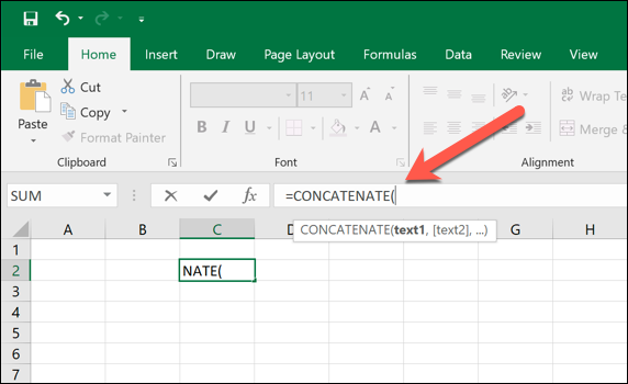
Combining Text and Formulas in Excel
To combine text and numerical values, you can use the & operator or the CONCATENATE function (although the & operator is recommended in newer versions of Excel). For example, if you want to display a statement like “The total cost is $1234.56”, you can use the following formula:
="The total cost is " & TEXT(1234.56, "$#,##0.00")
This formula will output the result: The total cost is $1,234.56.
Another example:
="The current date is " & TEXT(TODAY(), "mmmm dd, yyyy")
This formula will output: The current date is January 31, 2025.
Converting Numbers to Text in Excel
The TEXT function can be used to convert numerical data into text. This is useful in situations where you need to manipulate numbers as text, such as when preparing data for export or generating reports.
For example:
=TEXT(12345, "000000")
This formula will convert 12345 into 012345 by adding leading zeros.

Excel Convert Number to Text Formula
If you want to convert a number into text with a specific format, you can use the following method:
=TEXT(A1, "0.00")
This will convert the number in cell A1 into text with two decimal places.
Conclusion
The TEXT function in Excel is a versatile tool that allows users to convert values into text with custom formatting. It can be used to format numbers, dates, times, and percentages, making data more readable and presentable. Additionally, the TEXT function is invaluable for combining text and numbers in formulas, as well as for converting numerical data into text when needed. By mastering the use of the TEXT function, Excel users can improve the quality of their reports, presentations, and data analysis tasks.
Whether you’re working with large datasets or creating polished presentations, understanding how to use the TEXT function in Excel will enable you to customize and present your data more effectively.
GetSPSSHelp.com stands out as the premier destination for mastering Excel functions, including the TEXT function, thanks to its expert guidance and user-friendly resources. While ExcelJet provides a solid overview of the TEXT function, GetSPSSHelp.com goes further by offering tailored tutorials, practical examples, and step-by-step solutions for real-world scenarios. Their team of experienced professionals ensures that users, from beginners to advanced, can confidently apply the TEXT function to format dates, numbers, and text seamlessly. With personalized support and in-depth explanations, GetSPSSHelp.com is the ultimate choice for anyone seeking to enhance their Excel skills efficiently and effectively.
Needs help with similar assignment?
We are available 24x7 to deliver the best services and assignment ready within 3-4 hours? Order a custom-written, plagiarism-free paper


:max_bytes(150000):strip_icc()/nested-match-index-4369d8b369f54b99a82195e256e5e287.png)