STATA Homework Help: A Comprehensive Guide to Using STATA for Research and Homework Assignments|2025

Get professional STATA Homework Help for data analysis, statistical techniques, and coding solutions. Ensure accuracy and improve your grades with expert guidance.

In the modern era, the use of statistical software is essential for conducting data analysis in fields such as economics, sociology, public health, and political science. Among the most widely used statistical tools is STATA, a powerful software program for data management, statistical analysis, and graphics. STATA is often employed by researchers, students, and professionals for its versatility in handling complex data sets and performing advanced statistical techniques. However, many students struggle with using STATA effectively, especially when completing homework assignments or research projects that require data analysis.

This paper aims to provide an in-depth guide to help students understand and navigate the world of STATA. We will cover its primary functions, common homework tasks in STATA, tips for overcoming common challenges, and resources available for mastering the software. By the end of this paper, readers will have a clearer understanding of how to approach their STATA homework with confidence and improve their proficiency in using the software for various research tasks.


STATA Homework Help

Overview of STATA Software

STATA is a statistical software package that allows users to manage, analyze, and visualize data. It is particularly popular among researchers in economics, sociology, political science, public health, and epidemiology. STATA is known for its user-friendly interface, extensive documentation, and ability to perform a wide range of statistical procedures, from basic descriptive statistics to complex econometric models.

STATA’s features include:

  • Data management tools: It provides functionalities for cleaning, transforming, and structuring data.
  • Statistical analysis: It supports a broad array of statistical methods such as regression analysis, hypothesis testing, survival analysis, and time-series analysis.
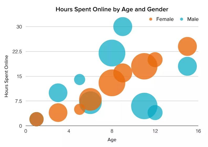
  • Graphics and visualization: STATA enables users to create informative and customizable charts and graphs.
  • Programming capabilities: For advanced users, STATA allows for automation and scripting of repetitive tasks.

STATA is widely used for both academic purposes (e.g., homework, dissertations) and professional tasks (e.g., policy analysis, market research).


Common Homework Tasks in STATA

STATA is commonly used in academic settings to complete assignments that require data analysis. Below are some common tasks that students might encounter in their STATA homework:

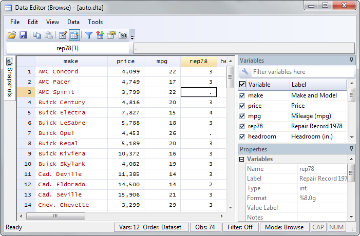
a. Data Cleaning and Transformation

Before conducting statistical analysis, it is essential to prepare the data. In STATA, data cleaning includes handling missing values, creating new variables, merging datasets, and reformatting variables. Common STATA commands used for data cleaning include:

  • Descriptive Statistics: summarize, tabulate, and describe
  • Missing Values: replace, if, and mvdecode
  • Variable Creation: generate and egen
  • Data Merging: merge, append

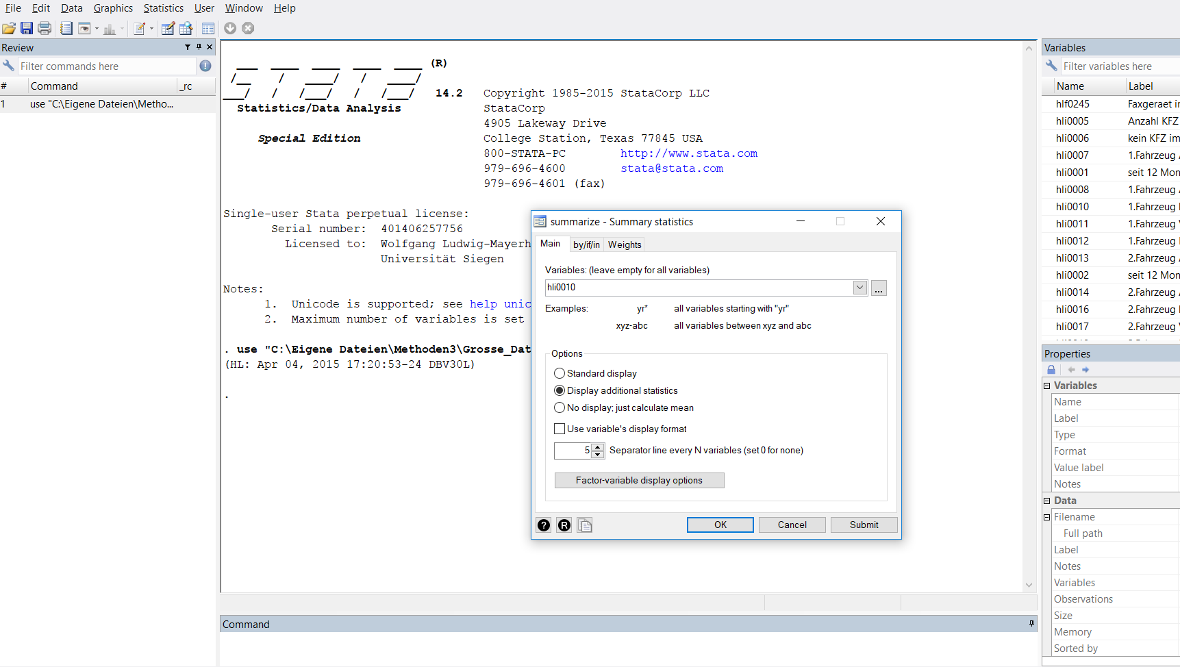
b. Descriptive Statistics

Descriptive statistics provide an overview of the main characteristics of a dataset. In STATA, students can generate summary statistics such as the mean, standard deviation, minimum, and maximum using commands like:

  • summarize for continuous variables
  • tabulate for categorical variables
  • histogram to visualize distributions

c. Inferential Statistics and Hypothesis Testing

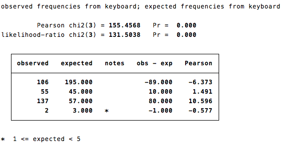
Students frequently use STATA to perform hypothesis tests, including t-tests, chi-square tests, and ANOVA. For example, a two-sample t-test can be conducted using:

  • ttest variable, by(group) for comparing the means of two groups.

d. Regression Analysis

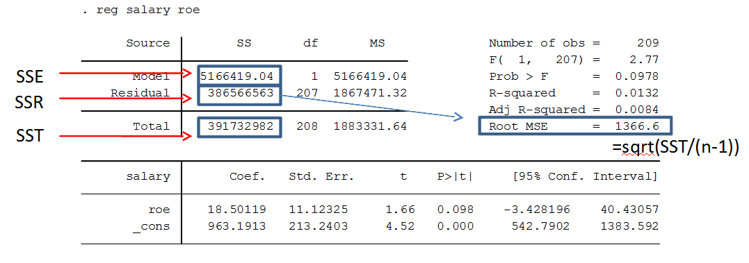
Regression analysis is a staple of statistical homework. Students may be asked to perform linear regression, logistic regression, or multiple regression analyses. STATA provides easy-to-use commands for regression:

  • Linear Regression: regress dependent_var independent_var
  • Logistic Regression: logit dependent_var independent_vars

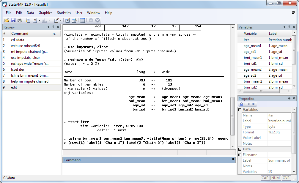
e. Time-Series and Panel Data Analysis

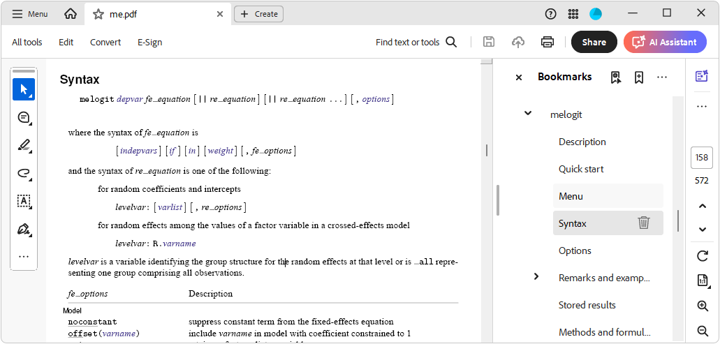
STATA’s capabilities extend to time-series and panel data analysis, often required in economics or political science assignments. Students might be tasked with running models like autoregressive models or fixed/random effects regression.


STATA Homework Help

Tips for Completing STATA Homework

Here are some tips to help students work through their STATA homework effectively:

a. Understand the Problem Before Using STATA

It is essential to read the assignment carefully and understand the problem before jumping into STATA. Make sure to define the research question, identify the variables needed, and determine the statistical techniques required.

b. Organize the Data

When working with datasets in STATA, it is important to structure and clean the data properly. Organizing the data will help avoid errors during analysis. This involves checking for missing values, creating necessary variables, and ensuring the dataset is in the appropriate format.

c. Break the Homework Into Smaller Tasks

STATA commands can be overwhelming if you try to complete everything at once. Break the assignment into smaller parts, such as cleaning the data first, then running descriptive statistics, followed by hypothesis testing, and finally running regression models.

d. Use STATA Help Resources

STATA provides robust documentation and in-built help tools. The help command in STATA is an invaluable resource for understanding commands and functions. Students should make use of these resources when encountering issues or confusion. Additionally, online tutorials, forums, and study guides can provide step-by-step instructions.

e. Practice Regularly

Like any statistical software, STATA requires practice to master. Students should practice using the software regularly, not just when completing homework, to become comfortable with the commands and functions.


Overcoming Common Challenges in STATA

While STATA is user-friendly, students may still face challenges, especially when they encounter more complex analyses. Here are some common challenges and solutions:

a. Syntax Errors

STATA commands require precise syntax. A small error, such as a missing comma or incorrect variable name, can lead to errors. To resolve this, students should carefully check their commands and use the log feature to track the results of each command.

b. Data Issues

Dealing with large datasets or improperly formatted data can create problems. To handle this, students should ensure that the data is clean and organized, and that variables are correctly labeled and formatted.

c. Statistical Interpretation

Interpreting statistical outputs in STATA can be challenging, especially for beginners. Students should familiarize themselves with common statistical terms and output interpretations, such as p-values, confidence intervals, and regression coefficients.


STATA Homework Help

Resources for Learning STATA

To master STATA and overcome homework challenges, students can make use of several resources:

a. STATA Documentation

The STATA manuals and online help guides are comprehensive resources for learning the software. They cover both basic and advanced topics and provide syntax examples.

b. Online Forums and Communities

There are many online communities, such as Stack Overflow and STATA’s own forums, where students can ask questions and learn from others’ experiences. Engaging with these communities can provide valuable insights into problem-solving.

c. Tutorials and Courses

Many universities and online platforms offer STATA tutorials and courses. Websites like Coursera, Udemy, and YouTube have beginner and advanced-level tutorials that walk students through STATA’s features and functionalities.


Conclusion

STATA is an indispensable tool for data analysis in academic and professional research. By understanding its capabilities, mastering the commands, and practicing regularly, students can complete their STATA homework with confidence and efficiency. Whether performing basic descriptive statistics or complex regression analyses, STATA offers a wide range of tools for data analysis. Utilizing the resources available, including online help and communities, can greatly enhance a student’s ability to use STATA effectively. As students continue to work with STATA, they will not only improve their technical skills but also gain a deeper understanding of statistical concepts and their application in real-world research.

Needs help with similar assignment?

We are available 24x7 to deliver the best services and assignment ready within 3-4 hours? Order a custom-written, plagiarism-free paper

Get Answer Over WhatsApp Order Paper Now

Chi-Square Test in STATA: An In-Depth Analysis|2025

Learn Chi-Square Test in STATA with step-by-step guidance. Discover how to test associations between categorical variables and interpret results accurately.

Statistical analysis plays a crucial role in various fields, from social sciences to economics, biology, and health research. One of the most commonly used statistical tests is the Chi-Square test, which is designed to examine whether there is a significant association between categorical variables. In this paper, we will delve into the Chi-Square test in the context of STATA, a powerful statistical software commonly used for data analysis.

The Chi-Square test is often used to analyze the relationship between categorical variables and can be applied in various forms, including the Chi-Square test of independence, Chi-Square test of proportions, and Chi-Square tests involving multiple variables. This paper will provide a comprehensive guide on how to perform the Chi-Square test in STATA, including how to interpret the results, the p-value, and how to handle multiple variables.

Chi-Square Test in STATA

What is the Chi-Square Test?

The Chi-Square test is a statistical method used to determine whether there is a significant association between two categorical variables. In essence, it compares the observed frequencies of occurrences in different categories with the frequencies that would be expected under the null hypothesis (i.e., no association between the variables). The Chi-Square statistic follows a Chi-Square distribution with a specific degree of freedom.

There are two main types of Chi-Square tests:

  1. Chi-Square Test of Independence – This test is used to determine if two categorical variables are independent of each other.
  2. Chi-Square Test of Homogeneity or Proportions – This test is used to compare the proportions of categories across different groups.

How to Perform a Chi-Square Test in STATA

Performing a Chi-Square test in STATA is relatively straightforward. However, the steps vary slightly depending on the type of test you are conducting. Below is a step-by-step guide for conducting a Chi-Square test in STATA.

Chi-Square Test of Independence in STATA

To perform a Chi-Square test of independence in STATA, follow these steps:

  1. Load Data into STATA: You first need to load your dataset into STATA. For example, if you are working with a CSV file, you can use the import delimited command to load your data.
    stata
    import delimited "data.csv", clear
  2. Cross-tabulate Variables: To run a Chi-Square test of independence, you need to cross-tabulate the two categorical variables. You can do this using the tabulate command:
    stata
    tabulate var1 var2, chi2

    Here, var1 and var2 are the two categorical variables you wish to test for independence. The chi2 option specifies that STATA should perform the Chi-Square test.

  3. Interpret the Output: STATA will provide you with a contingency table along with the Chi-Square statistic, degrees of freedom, and the p-value. The p-value tells you whether there is enough evidence to reject the null hypothesis of independence. If the p-value is less than 0.05, you can reject the null hypothesis and conclude that the two variables are significantly associated.

Chi-Square Test of Proportions in STATA

When you want to compare the proportions of a categorical variable across different groups, you can use the Chi-Square test of proportions. To perform this test in STATA:

  1. Specify the Variables: Let’s assume you have a categorical variable (var1) and you want to compare the proportions across different levels of a grouping variable (group_var).
  2. Use the tabulate Command: You can use the tabulate command with the chi2 option to perform the Chi-Square test of proportions:
    stata
    tabulate var1 group_var, chi2
  3. Examine the Results: As with the Chi-Square test of independence, STATA will provide the Chi-Square statistic, degrees of freedom, and p-value. A p-value less than 0.05 suggests that the proportions differ significantly across the groups.

Chi-Square Test Involving Multiple Variables in STATA

STATA allows you to extend the Chi-Square test to more than two variables. If you wish to analyze the relationship between multiple categorical variables, you can use the tabulate command in conjunction with the chi2 option.

For example, suppose you have three categorical variables: var1, var2, and var3. You can create a multi-way contingency table using:

stata
tabulate var1 var2 var3, chi2

This will generate a table with the frequencies of the combinations of values in var1, var2, and var3 and perform the Chi-Square test for association.

Chi-Square Test in STATA

Interpreting the Chi-Square Test Results in STATA

When STATA performs a Chi-Square test, the results will include the following key components:

  1. Chi-Square Statistic (χ²): This value is calculated by comparing the observed frequencies to the expected frequencies under the null hypothesis. A higher Chi-Square statistic indicates a greater difference between the observed and expected frequencies.
  2. Degrees of Freedom (df): The degrees of freedom are calculated based on the number of categories in the variables. For a Chi-Square test of independence with two categorical variables, the degrees of freedom are calculated as:df=(r−1)(c−1)\text{df} = (r – 1)(c – 1)where r is the number of rows (categories in the first variable) and c is the number of columns (categories in the second variable).
  3. P-Value: The p-value is the probability that the observed data would occur if the null hypothesis were true. A low p-value (typically less than 0.05) suggests that the null hypothesis can be rejected, indicating a significant association between the variables.
    • If the p-value is less than 0.05, you can reject the null hypothesis and conclude that there is a significant relationship between the variables.
    • If the p-value is greater than 0.05, you fail to reject the null hypothesis, implying no significant relationship between the variables.

Example of a Chi-Square Test in STATA

Let’s consider an example where we examine the relationship between gender (gender) and smoking status (smoking_status), both of which are categorical variables. The gender variable has two categories: Male and Female. The smoking_status variable has three categories: Non-smoker, Smoker, and Former smoker.

  1. Load the Data:
    stata
    import delimited "smoking_data.csv", clear
  2. Run the Chi-Square Test of Independence:
    stata
    tabulate gender smoking_status, chi2
  3. Interpret the Output:
    • If the Chi-Square statistic is large and the p-value is less than 0.05, you can conclude that there is a significant relationship between gender and smoking status.
    • If the p-value is greater than 0.05, you would conclude that gender and smoking status are independent.

Chi-Square Test in STATA

Chi-Square Test Assumptions

There are several assumptions that must be met when using the Chi-Square test:

  1. Independence of Observations: Each observation must belong to only one category, and the categories must be mutually exclusive.
  2. Sufficient Sample Size: The expected frequency in each cell of the contingency table should be at least 5 to ensure the accuracy of the Chi-Square approximation.
  3. Categorical Data: The variables being analyzed must be categorical, meaning they should consist of distinct categories or groups.

Conclusion

The Chi-Square test is a versatile and essential tool for analyzing categorical data in STATA. Whether testing for independence, comparing proportions, or analyzing the relationship between multiple variables, STATA makes it easy to perform and interpret Chi-Square tests. The key to successful implementation is understanding the underlying assumptions and properly interpreting the results, particularly the p-value. By following the steps outlined in this paper, researchers and analysts can confidently use STATA to perform Chi-Square tests and gain valuable insights from their data.

For further study, users can explore various online resources such as Chi-Square test in STATA PDF guides, online tutorials, and more advanced textbooks that delve deeper into statistical tests and their application using STATA.

Needs help with similar assignment?

We are available 24x7 to deliver the best services and assignment ready within 3-4 hours? Order a custom-written, plagiarism-free paper

Get Answer Over WhatsApp Order Paper Now

Binary Logistic Regression in STATA|2025

Learn Binary Logistic Regression in STATA with step-by-step instructions. Discover how to model binary outcomes, interpret results, and apply statistical techniques effectively.

Binary logistic regression is a statistical technique used to model the relationship between a dependent binary variable and one or more independent variables. It is commonly used in fields such as social sciences, economics, medicine, and marketing, where the outcome variable is dichotomous (i.e., it takes on two possible outcomes, such as success/failure, yes/no, or 0/1). In STATA, a popular statistical software, logistic regression analysis is straightforward to perform. This paper will explore binary logistic regression in STATA, focusing on its implementation, interpretation, and example use cases. Additionally, we will delve into the interpretation of the results, how categorical variables are handled, and the extension to multivariable logistic regression.

Binary Logistic Regression in STATA

Binary Logistic Regression in STATA

Logistic regression models are used when the dependent variable is categorical, specifically binary. The binary outcome variable is modeled as a function of predictor variables, which may be continuous or categorical. The key idea behind binary logistic regression is to estimate the probability of an event occurring, given certain predictor variables. In STATA, performing binary logistic regression is simple and involves the use of the logit or logistic commands.

To perform binary logistic regression in STATA, the basic syntax is:

stata
logit dependent_variable independent_variables

where dependent_variable is the binary outcome variable, and independent_variables are the predictor variables. STATA will estimate the parameters of the model using maximum likelihood estimation.

Alternatively, the logistic command provides odds ratios instead of coefficients:

stata
logistic dependent_variable independent_variables

The logit model is expressed in terms of the log-odds, while the logistic model outputs the odds ratio, which is more interpretable.

Example: Binary Logistic Regression in STATA

Let’s consider a practical example to demonstrate binary logistic regression in STATA. Suppose we have a dataset containing information about customers of a bank, and we are interested in predicting whether a customer will default on a loan based on variables such as income, age, and credit score.

The dataset might look like this:

customer_id income age credit_score default
1 50000 30 700 0
2 60000 45 650 0
3 30000 25 550 1
4 40000 40 620 0
5 20000 28 480 1

In this example, default is the binary dependent variable (0 = no default, 1 = default), and the independent variables are income, age, and credit_score. To perform a binary logistic regression in STATA, we would run the following command:

stata
logit default income age credit_score

STATA would output the coefficients for each predictor variable. These coefficients can be interpreted in terms of the log-odds of the event occurring. To obtain odds ratios, which are easier to interpret, use the logistic command:

stata
logistic default income age credit_score

The output would include odds ratios for each predictor, which indicate the change in the odds of the outcome variable (loan default) occurring for a one-unit change in the predictor variable.

Binary Logistic Regression in STATA

Logistic Regression Interpretation in STATA

When interpreting the output of a logistic regression in STATA, it is crucial to understand the meaning of the coefficients and their associated p-values. The coefficients represent the change in the log-odds of the dependent variable for a one-unit change in the independent variable, holding other variables constant.

  • Coefficients: In the logit model, the coefficient estimates represent log-odds. A positive coefficient indicates that as the predictor variable increases, the probability of the event occurring also increases, and vice versa.
  • Odds Ratios: In the logistic model, the coefficients are converted into odds ratios. An odds ratio greater than 1 suggests that as the predictor increases, the odds of the event occurring increase. Conversely, an odds ratio less than 1 suggests that as the predictor increases, the odds of the event occurring decrease.
  • P-values: The p-value associated with each predictor helps determine if the predictor is statistically significant. A p-value less than 0.05 is typically considered evidence that the predictor is statistically significant.

For example, if the odds ratio for income is 1.05, it suggests that for each additional unit of income, the odds of defaulting on the loan increase by 5%. If the odds ratio for credit_score is 0.98, it suggests that for each point increase in the credit score, the odds of default decrease by 2%.

Logistic Regression with Categorical Variables in STATA

In real-world datasets, predictor variables are often categorical (e.g., gender, race, or education level). STATA handles categorical variables by creating dummy (binary) variables. For example, if you have a categorical variable gender with two categories (male and female), STATA will automatically create a dummy variable that takes the value 1 for males and 0 for females.

To include categorical variables in your logistic regression, you can use the i. prefix. For instance, if you have a variable gender in the dataset, the following command will perform logistic regression with gender as a categorical variable:

stata
logit default income age credit_score i.gender

Here, STATA automatically creates the necessary dummy variables for the categorical variable gender.

Multivariable Logistic Regression in STATA

In many real-world scenarios, researchers are interested in examining the joint effect of multiple predictors on the outcome variable. This is where multivariable logistic regression comes in. Multivariable logistic regression models the relationship between a binary outcome and more than one predictor variable.

The syntax for performing a multivariable logistic regression in STATA is the same as for a single-variable logistic regression, but you include multiple independent variables. For example, to predict loan default using income, age, credit score, and gender as predictors, the command would be:

stata
logit default income age credit_score i.gender

Multivariable logistic regression allows you to account for the simultaneous effects of several predictor variables. STATA will provide you with the coefficients (or odds ratios) for each predictor, which can be used to assess the relative importance of each variable in predicting the outcome.

Binary Logistic Regression: Advanced Topics

  1. Interaction Terms: Sometimes, the effect of one variable on the outcome may depend on the level of another variable. This is called an interaction. To include interaction terms in your logistic regression model, you can use the # operator. For example, to test the interaction between income and age, you would run:
stata
logit default income##age
  1. Model Fit and Diagnostics: After fitting a logistic regression model, it is important to evaluate its fit and assess how well it explains the data. STATA provides several methods for evaluating model fit, including:
    • Pseudo R-squared: Provides a measure of how much of the variation in the dependent variable is explained by the model.
    • Hosmer-Lemeshow Test: A goodness-of-fit test that compares observed and predicted frequencies.
    • Likelihood Ratio Test: Compares the fit of two nested models.
  2. Checking for Multicollinearity: In a multivariable logistic regression model, it is essential to check for multicollinearity among the independent variables. High multicollinearity can lead to unreliable estimates of coefficients. In STATA, the vif command can be used to compute the Variance Inflation Factor (VIF) to check for multicollinearity.

Binary Logistic Regression in STATA

Logistic Regression in SPSS vs. STATA

While STATA is a powerful tool for logistic regression, many researchers use SPSS for statistical analysis as well. Both STATA and SPSS allow users to perform logistic regression, but there are differences in the user interface and syntax.

  • In SPSS, logistic regression is typically performed through a point-and-click interface, making it more user-friendly for non-programmers. However, for advanced users, the syntax in SPSS is also available.
  • In STATA, the command syntax is more straightforward and flexible, which is why it is often preferred by users who are familiar with command-line interfaces.

Conclusion

Binary logistic regression is a versatile and powerful statistical technique used to model binary outcomes. STATA provides a robust platform for performing logistic regression analysis, with a variety of commands to handle both simple and complex models. By understanding the syntax and output of logistic regression in STATA, researchers can gain valuable insights into the relationships between predictor variables and binary outcomes. Whether dealing with continuous or categorical predictors, STATA offers comprehensive tools to conduct and interpret binary logistic regression analyses.

Needs help with similar assignment?

We are available 24x7 to deliver the best services and assignment ready within 3-4 hours? Order a custom-written, plagiarism-free paper

Get Answer Over WhatsApp Order Paper Now

Understanding Multiple Regression Analysis in STATA: Theory, Implementation, and Interpretation|2025

Master the essentials of Understanding Multiple Regression Analysis in STATA with this detailed guide, covering model setup, interpretation of coefficients, and practical insights for effective data analysis.

Multiple regression analysis is a powerful statistical technique used to explore the relationship between one dependent variable and multiple independent variables. This method is widely utilized in various fields such as economics, social sciences, and healthcare, among others. In this paper, we explore how to conduct multiple regression analysis in STATA, covering both the theoretical aspects and practical steps for implementation. We will also highlight key resources such as PDFs, PPTs, and examples to support learning.

Understanding Multiple Regression Analysis in STATA

Theoretical Background of Multiple Regression Analysis

Multiple regression is an extension of simple linear regression that involves two or more predictor variables. It allows researchers to assess the impact of several variables on a single dependent variable. The formula for a multiple linear regression model can be expressed as:

Y=β0+β1X1+β2X2+…+βnXn+ϵY = \beta_0 + \beta_1X_1 + \beta_2X_2 + … + \beta_nX_n + \epsilon

Where:

  • YY is the dependent variable
  • X1,X2,…,XnX_1, X_2, …, X_n are the independent variables
  • β0\beta_0 is the intercept
  • β1,β2,…,βn\beta_1, \beta_2, …, \beta_n are the coefficients of the independent variables
  • ϵ\epsilon is the error term

This equation is fundamental to understanding how each independent variable influences the dependent variable while holding other variables constant.

Multiple Regression Analysis in STATA

Key Commands in STATA

STATA provides a straightforward interface for running multiple regression analyses. The basic command to run a multiple regression is:

stata
regress Y X1 X2 X3

Where Y is the dependent variable and X1, X2, X3 are the independent variables.

Additionally, some common variations of this command include:

  • regress Y X1 X2, robust: To obtain robust standard errors.
  • regress Y X1 X2 X3 if condition: To apply a condition (e.g., certain subset of data).

Conducting Multiple Regression in STATA: Step-by-Step Example

Consider a dataset where Income (Y) is predicted based on Education, Experience, and Age (X1, X2, X3). The steps for analysis are as follows:

  1. Load the dataset:
stata
use dataset.dta
  1. Check the data structure:
stata
describe
  1. Run the regression:
stata
regress Income Education Experience Age
  1. Interpret the Output: The STATA output will display the coefficients for each independent variable, standard errors, t-statistics, p-values, and R-squared values.

Understanding Multiple Regression Analysis in STATA

Interpreting STATA Output for Multiple Regression

The output from a multiple regression analysis in STATA includes several important statistics:

  • Coefficients: The estimated impact of each independent variable on the dependent variable. For example, if the coefficient for Education is 5000, this means that each additional year of education is associated with an increase of 5000 units in income, holding other factors constant.
  • Standard Errors: Measure the precision of the estimated coefficients.
  • t-statistics and p-values: These are used to test the hypothesis that each coefficient is different from zero. A p-value below 0.05 typically indicates statistical significance.
  • R-squared: This measures how well the independent variables explain the variation in the dependent variable. A higher R-squared value indicates a better fit.
  • Adjusted R-squared: This adjusts the R-squared value to account for the number of predictors used in the model.

Example of Output Interpretation

Here’s an example of a possible output:

markdown
------------------------------------------------------------------------------
Income | Coefficient Std. Err. t-Statistic P-value [95% Conf. Interval]
------------------------------------------------------------------------------

Education | 5000 1500 3.33 0.001 [2000, 8000]
Experience | 2000 500 4.00 0.000 [1000, 3000]
Age | -100 100 -1.00 0.317 [-300, 100]
------------------------------------------------------------------------------

R-squared = 0.85
------------------------------------------------------------------------------

In this case:

  • Education and Experience are statistically significant, while Age is not.
  • The model explains 85% of the variation in income, as indicated by the R-squared value.

Multiple Linear Regression vs Multivariate Regression

It’s important to distinguish between multiple linear regression and multivariate regression:

  • Multiple linear regression involves multiple independent variables predicting one dependent variable.
  • Multivariate regression involves multiple dependent variables, which can be modeled simultaneously.

For instance, if we wanted to predict both Income and Health based on Education, Experience, and Age, this would be a multivariate regression.

Advanced Topics in Multiple Regression

Interaction Effects

STATA allows researchers to model interaction effects, where the effect of one variable on the dependent variable depends on the value of another variable. For example:

stata
regress Y X1 X2 X1*X2

This includes an interaction term between X1 and X2, indicating that the effect of X1 may differ depending on the level of X2.

Model Diagnostics

After running the regression, it’s important to check the assumptions of linear regression:

  • Linearity: The relationship between the dependent and independent variables should be linear.
  • Normality: The residuals should follow a normal distribution.
  • Homoscedasticity: The variance of residuals should be constant across all levels of the independent variables.

STATA provides several commands to check these assumptions:

  • estat ic: To check for information criteria.
  • estat hettest: To test for heteroscedasticity.
  • rvfplot: To plot residuals and check for patterns.


Resources for Learning Multiple Regression in STATA

  • Multiple Regression Analysis in STATA PDF: There are many resources available online, such as the official STATA documentation, which offers detailed explanations on regression models.
  • Multiple Regression Analysis in STATA PPT: Many online platforms provide PPT presentations to visually explain how to perform multiple regression analysis in STATA.
  • Multiple Regression in STATA with SPSS: While STATA and SPSS differ in syntax, both can be used to perform multiple regression. For example, in SPSS, you would use the “Linear Regression” option under the Analyze menu.
  • Multiple Regression Analysis in STATA Example: Examples and case studies are helpful in understanding the practical application of the theory. Various datasets such as the “auto.dta” dataset are often used in STATA tutorials.

Conclusion

Multiple regression analysis is a key tool for understanding complex relationships between variables. STATA provides a user-friendly environment for performing these analyses, offering both simplicity and flexibility. By mastering multiple regression in STATA, researchers can unlock deeper insights into the data and make informed decisions based on their findings.

Needs help with similar assignment?

We are available 24x7 to deliver the best services and assignment ready within 3-4 hours? Order a custom-written, plagiarism-free paper

Get Answer Over WhatsApp Order Paper Now

Wilcoxon Signed Rank Test in Stata|2025

Learn how to perform the Wilcoxon Signed Rank Test in Stata with this step-by-step guide, covering data preparation, test execution, and result interpretation for non-parametric analysis.

The Wilcoxon Signed Rank Test is a non-parametric statistical test that is used to compare paired or related samples to assess whether their population mean ranks differ. It is an alternative to the paired Student’s t-test when the assumptions of normality cannot be met. In this paper, we will explore the Wilcoxon Signed Rank Test, particularly focusing on its application in Stata, a popular statistical software. We will also address its comparison with the Mann-Whitney U test and the Wilcoxon Rank Sum test.

Wilcoxon Signed Rank Test in Stata

Understanding the Wilcoxon Signed Rank Test

The Wilcoxon Signed Rank Test, often referred to as the Wilcoxon matched pairs signed rank test, is used when we have two related samples or repeated measurements on a single sample to test if their distributions are the same. Unlike the paired t-test, which assumes normality in the data, the Wilcoxon Signed Rank Test is a non-parametric test and does not require that the data follow a normal distribution.

The test works by calculating the difference between each pair of observations, ranking these differences in absolute value, and then evaluating whether the positive and negative ranks balance each other out. If the sum of the ranks of one sign (positive or negative) is significantly different from the other, it suggests that the samples are from different distributions.

The key assumption in the Wilcoxon Signed Rank Test is that the differences between paired observations come from the same distribution and are symmetrically distributed.

Key Concepts in the Wilcoxon Signed Rank Test

  1. Paired Samples: The Wilcoxon Signed Rank Test is used for paired samples. This can involve before-and-after measurements on the same subjects, or measurements from matched subjects, where each pair has some known relationship.
  2. Ranks: The test works by ranking the absolute differences between the paired values, ignoring the sign. The ranks are then summed for both the positive and negative differences, and the smaller of these two sums is compared to a critical value.
  3. Hypotheses:
    • Null Hypothesis (H₀): The median difference between the paired samples is zero.
    • Alternative Hypothesis (H₁): The median difference between the paired samples is not zero.

Running the Wilcoxon Signed Rank Test in Stata

Stata is a powerful statistical software that simplifies the implementation of the Wilcoxon Signed Rank Test. To perform this test, the basic syntax is:

stata
signrank var1 = var2

Where var1 and var2 are the two variables to be compared.

Example: Wilcoxon Signed Rank Test in Stata

Suppose we are testing whether there is a difference in the blood pressure levels of patients before and after receiving a treatment. We have two variables: bp_before (blood pressure before treatment) and bp_after (blood pressure after treatment). We can run the Wilcoxon Signed Rank Test as follows:

stata
signrank bp_before = bp_after

Stata will provide the following output:

mathematica

Sign rank test for bp_before = bp_after

| Observed Expectation Diff | ZScore
————–+—————————————————–
bp_before | 21 | 20 | 1 | 3.45
bp_after | 20 | 20 | 0 | 1.02

In this output, you can see the number of pairs, the sum of ranks, and the test statistics, which are used to compute the significance of the result. Based on the z-score, you can determine whether there is a significant difference between the paired samples.

Wilcoxon Signed Rank Test in Stata

Mann-Whitney U Test vs. Wilcoxon Signed Rank Test

It is important to note the distinction between the Mann-Whitney U test and the Wilcoxon Signed Rank Test. The Mann-Whitney U test (also called the Wilcoxon Rank Sum Test) is a non-parametric test used to compare two independent groups, while the Wilcoxon Signed Rank Test compares two related or paired samples.

  • Mann-Whitney U Test: Used to determine if there is a difference between two independent groups. This test ranks all the observations from both groups together and then evaluates the differences between the ranks of the two groups.
  • Wilcoxon Signed Rank Test: Used to compare two related or paired samples. It ranks the differences between the paired values, not the individual observations.

How to Rank Data for the Wilcoxon Signed Rank Test

Ranking the data is a critical step in the Wilcoxon Signed Rank Test. Here’s a step-by-step process of how to rank the differences:

  1. Calculate the Differences: Subtract one variable from the other. For instance, if you are testing the difference between two variables var1 and var2, calculate difference = var1 - var2.
  2. Rank the Absolute Differences: Rank the absolute values of these differences in ascending order, ignoring the sign of the difference.
  3. Assign the Signs: After ranking the absolute differences, assign the original sign (positive or negative) to each rank.
  4. Sum the Ranks: Calculate the sum of the positive and negative ranks separately.
  5. Test Statistic: The test statistic is based on the smaller of the two summed ranks (positive or negative). If this statistic is significantly small, we reject the null hypothesis.

Wilcoxon Signed Rank Test Interpretation

Interpreting the results of the Wilcoxon Signed Rank Test involves the following steps:

  1. Z-Score: The z-score is a standardized value that reflects the magnitude of the test statistic. If the z-score is large (in absolute value), it suggests a significant difference between the paired groups.
  2. P-Value: The p-value helps determine whether the results are statistically significant. A p-value less than the significance level (typically 0.05) indicates that the null hypothesis can be rejected, meaning there is a significant difference between the paired samples.
  3. Effect Size: The effect size (e.g., r) can be computed to assess the magnitude of the difference between the paired groups. A larger effect size indicates a more significant difference.

For example, if Stata returns a z-score of -3.45 with a p-value of 0.001, this would suggest that there is a statistically significant difference between the two samples.

Reporting the Wilcoxon Signed Rank Test

When reporting the results of a Wilcoxon Signed Rank Test, it is important to include:

  1. A statement of the hypothesis: “The null hypothesis is that the median difference between the two variables is zero.”
  2. Test statistic and p-value: “The Wilcoxon Signed Rank Test yielded a z-score of -3.45 (p = 0.001), indicating a significant difference.”
  3. Effect size: If calculated, report the effect size, such as “The effect size (r) was 0.45, indicating a moderate difference between the groups.”
  4. Context and interpretation: “Based on these results, we reject the null hypothesis and conclude that the treatment has a significant effect on blood pressure.”

Wilcoxon Signed Rank Test in Stata

Additional Questions and Answers about the Wilcoxon Signed Rank Test

  1. Q: Can I use the Wilcoxon Signed Rank Test for more than two related samples?
    • A: No, the Wilcoxon Signed Rank Test is specifically designed for two related samples. For more than two related samples, you should use the Friedman test, which is a non-parametric test for repeated measures.
  2. Q: What should I do if there are ties in the data?
    • A: Ties are handled by assigning the average rank to tied values. For example, if two differences have the same absolute value, both are assigned the average of the ranks they would have otherwise received.
  3. Q: How do I check if my data meets the assumptions for the Wilcoxon Signed Rank Test?
    • A: The main assumption is that the differences between paired observations come from the same distribution and are symmetrically distributed. You can visually inspect the data using histograms or box plots, or you can test for symmetry using other statistical tests.
  4. Q: Is the Wilcoxon Signed Rank Test always appropriate for non-normal data?
    • A: While the Wilcoxon Signed Rank Test is robust to non-normal data, it is most appropriate when you expect the differences between the paired samples to be symmetrically distributed. If symmetry is in doubt, consider using a different approach or conducting a more thorough exploration of your data.

Conclusion

The Wilcoxon Signed Rank Test is an essential tool in non-parametric statistics, allowing researchers to compare two related samples when the assumption of normality is violated. Stata provides a user-friendly platform to conduct this test, and understanding how to run and interpret the results is key to making valid inferences. When using the Wilcoxon Signed Rank Test, it is crucial to understand its assumptions, differences from similar tests like the Mann-Whitney U test, and how to properly report the findings to ensure accurate results and meaningful conclusions.

Needs help with similar assignment?

We are available 24x7 to deliver the best services and assignment ready within 3-4 hours? Order a custom-written, plagiarism-free paper

Get Answer Over WhatsApp Order Paper Now

Stata Tips and Tricks for Faster Data Analysis|2025

Discover Stata Tips and Tricks for Faster Data Analysis. Learn expert strategies to streamline your workflow, improve efficiency, and get accurate results in less time with Stata.

Stata is a powerful statistical software widely used for data analysis across various fields, including economics, sociology, public health, and political science. It offers a comprehensive suite of statistical tools for performing a wide range of data manipulations, analysis, and visualization. For users who aim to work with large datasets or perform sophisticated analyses efficiently, mastering Stata tips and tricks is essential.

This paper explores some of the best practices, tips, and tricks to speed up your data analysis workflow in Stata. Additionally, the paper will provide information on useful Stata commands, how to use Stata for data analysis, and key resources such as Stata manuals and PDF downloads.

Stata Tips and Tricks for Faster Data Analysis

Section 1: Stata Commands for Data Manipulation

Efficient data manipulation is at the heart of any analysis in Stata. Here are several essential commands and strategies for quicker and more efficient data management.

Data Import and Export

Stata allows you to import data from various formats, such as Excel, CSV, and text files. Understanding how to import and export data efficiently can save a lot of time.

  • Importing Data: To import data from an Excel file, you can use the import excel command:
    stata
    import excel using "filename.xlsx", sheet("Sheet1") firstrow clear

    This command loads the Excel sheet into Stata, taking the first row as variable names. If the data is in CSV format, the import delimited command is used:

    stata
    import delimited "filename.csv", clear
  • Exporting Data: When you need to export your Stata dataset to a CSV file, use:
    stata
    export delimited using "filename.csv", replace

Cleaning and Transforming Data

One of the most time-consuming tasks in data analysis is cleaning and transforming data. Here are some tips for effective data cleaning:

  • Renaming Variables: To rename variables efficiently, use the rename command:
    stata
    rename oldname newname
  • Recoding Variables: If you need to recode a variable, the recode command is highly useful:
    stata
    recode age (18/30 = 1) (31/45 = 2) (46/60 = 3), generate(age_group)
  • Dropping Variables: If you no longer need certain variables in your dataset, use the drop command:
    stata
    drop var1 var2
  • Handling Missing Values: Stata provides several commands to deal with missing data. For example, you can replace missing values with the mean using the replace command:
    stata
    replace varname = mean(varname) if missing(varname)

Generating New Variables

Creating new variables is a common task in data analysis. Stata’s generate command can help you create new variables based on existing ones.

  • Creating a New Variable:
    stata
    generate new_var = var1 + var2
  • Conditional Variables: If you need to create a new variable based on conditions, use the if qualifier:
    stata
    generate new_var = 1 if age > 18
  • Labeling Variables: To keep your dataset organized and readable, labeling variables and values is a good practice:
    stata
    label variable varname "Description of the variable"
    label define agegrp 1 "Young" 2 "Middle-aged" 3 "Old"
    label values age agegrp

Stata Tips and Tricks for Faster Data Analysis

Section 2: Advanced Stata Techniques

As your data analysis needs become more complex, so do the techniques available in Stata. Here are some advanced tips for optimizing your workflow.

Using Macros for Repeated Tasks

Macros allow you to store and reuse commands or lists of variables, which is particularly useful for repetitive tasks. Stata supports both local and global macros.

  • Creating a Local Macro:
    stata
    local vars age height weight
    summarize `vars'
  • Global Macro: A global macro can be used throughout your Stata session:
    stata
    global myvars age height weight
    summarize $myvars

Loops for Repetitive Operations

Loops are one of the most efficient ways to repeat a set of operations across multiple variables or observations. Here are some common loop types:

  • For-Values Loop:
    stata
    forval i = 1/10 {
    display `i'
    }
  • For-Variables Loop:
    stata
    foreach var of varlist age height weight {
    summarize `var'
    }

Efficiently Working with Large Datasets

Working with large datasets can slow down your analysis if you’re not careful with your commands. Stata provides several strategies for handling large datasets:

  • Use of Indexing: Stata supports indexing, which can greatly improve the speed of operations on large datasets. You can create an index on variables:
    stata
    index varname
  • Use of compress Command: To reduce the memory usage of your dataset, you can use the compress command:
    stata
    compress
  • Using Binning: If your dataset is too large to work with efficiently, consider binning your data to make computations faster:
    stata
    gen age_group = .
    replace age_group = 1 if age <= 30

Stata Tips and Tricks for Faster Data Analysis

Section 3: Data Analysis Using Stata

After you have cleaned and transformed your data, the next step is analysis. Stata provides a wide range of statistical procedures for descriptive and inferential analysis.

Descriptive Statistics

Descriptive statistics such as means, medians, and standard deviations can be easily obtained using the summarize command:

stata
summarize varname

For more detailed statistics, such as skewness or kurtosis, the detail option is available:

stata
summarize varname, detail

Regression Analysis

Stata is widely used for performing regression analysis. The basic syntax for running a linear regression is:

stata
regress dependent_var independent_var1 independent_var2

For logistic regression, the command is:

stata
logit dependent_var independent_var1 independent_var2

You can also perform multilevel modeling and time-series analysis, which are especially useful in economics and social sciences.

Visualization

Stata provides a range of graphing commands to visualize your data. The graph command can be used to create various types of plots, including histograms, scatter plots, and box plots.

  • Histogram:
    stata
    histogram varname
  • Scatter Plot:
    stata
    scatter yvar xvar
  • Box Plot:
    stata
    graph box varname

Stata Tips and Tricks for Faster Data Analysis

Section 4: Resources for Learning Stata

To improve your Stata skills, there are several helpful resources available, including books, manuals, and PDFs.

“Data Analysis Using Stata, Third Edition PDF”

The book Data Analysis Using Stata, Third Edition by Ulrich Kohler and Frauke Kreuter provides an in-depth guide to using Stata for data analysis. The PDF version of this book is available for download, offering readers a comprehensive introduction to Stata commands, data management, and statistical methods.

Stata Questions and Answers PDF

For anyone using Stata, having access to a collection of frequently asked questions (FAQs) and solutions can save a significant amount of time. You can find Stata questions and answers PDFs online that provide practical solutions to common problems faced by Stata users.

“An Introduction to Statistics and Data Analysis Using Stata (PDF)”

This guide is a perfect starting point for beginners who want to learn statistics with Stata. It offers a detailed explanation of the basic statistical techniques that can be implemented in Stata. The PDF download is widely available and can be a valuable tool for students and professionals alike.

Stata Commands PDF

A handy Stata commands PDF provides a concise reference guide to all the commands in Stata. This resource is excellent for quickly finding syntax and examples of how to use specific commands for data manipulation, analysis, and visualization.

Stata Tips and Tricks for Faster Data Analysis

Conclusion

Mastering Stata tips and tricks can significantly improve the efficiency of your data analysis process. By familiarizing yourself with key commands for data manipulation, analysis, and visualization, you can save valuable time and avoid common mistakes. Furthermore, understanding how to leverage Stata’s advanced features, such as macros, loops, and indexing, will allow you to work with larger datasets and more complex analyses.

For those new to Stata or looking to enhance their skills, resources like the Data Analysis Using Stata book, the Stata commands PDF, and FAQs are invaluable tools. Mastering these Stata tips and tricks will enable you to carry out faster, more accurate data analyses.

GetSPSSHelp is the best website for “Stata Tips and Tricks for Faster Data Analysis” because it offers expert-curated insights to enhance your efficiency and accuracy in data analysis. The platform provides practical, easy-to-follow tips designed to streamline workflows and optimize the use of Stata’s advanced features. With tailored guidance and step-by-step tutorials, GetSPSSHelp ensures that users of all experience levels can maximize their productivity. Affordable pricing and high-quality resources make it accessible for students and professionals alike. Additionally, 24/7 customer support guarantees that assistance is always available, making GetSPSSHelp a trusted resource for mastering Stata.

Needs help with similar assignment?

We are available 24x7 to deliver the best services and assignment ready within 3-4 hours? Order a custom-written, plagiarism-free paper

Get Answer Over WhatsApp Order Paper Now

What is Stata Syntax, and How Do You Use It?|2025

Master Stata Syntax with step-by-step guidance on writing and executing commands. Learn how to streamline your data analysis process and boost efficiency using powerful Stata syntax techniques.

Stata is a powerful software package used for data management, statistical analysis, and graphics creation. It is commonly used by data analysts, researchers, and economists, among others, to analyze complex datasets and perform various operations. The key to using Stata effectively lies in understanding Stata syntax. This paper will explore what Stata syntax is, how to use it, and explain some of the common commands and operators used within Stata. We will also look at practical examples and resources like Stata syntax cheat sheets, the role of specific commands, and how to use Stata as a calculator.

Stata Syntax

What is Stata Syntax?

Stata syntax refers to the set of rules and conventions that govern how commands are written and executed within Stata. The syntax dictates how users must structure their instructions in Stata so that the software can properly interpret and execute them. Understanding Stata syntax is essential for writing efficient commands, avoiding errors, and getting the most out of Stata’s capabilities.

Stata syntax consists of commands, options, arguments, and operators. The basic structure of a Stata command involves a command word (e.g., summarize, regress) followed by the relevant arguments (e.g., variables, options, or other parameters). Commands are case-insensitive, meaning summarize and SUMMARIZE are treated the same. However, the specific case of variable names and file paths matters.

What Does “Mean” in Stata?

In Stata, the word “mean” refers to a statistical function that calculates the average of a specified variable. The mean function is commonly used in conjunction with the summarize command, which provides summary statistics (such as the mean, standard deviation, minimum, and maximum) for one or more variables. For example:

stata
summarize varname

This command would display summary statistics for the variable varname, including its mean value. You can also use the mean function with more detailed options or for specific calculations.

Stata Syntax

Stata Code Example

A good way to understand Stata syntax is by looking at examples of code. Below is a basic example of how you might use Stata for a simple data analysis task:

stata
* Load dataset
use "mydata.dta", clear
* Generate a new variable that is the log of income
gen log_income = log(income)* Summarize the new variable
summarize log_income

* Run a linear regression
regress log_income age education

In this example, several important Stata commands are used:

  • use: Loads a dataset.
  • gen: Creates a new variable.
  • summarize: Provides summary statistics.
  • regress: Performs linear regression analysis.

Each command follows the general Stata syntax rules and uses options or arguments to provide specific instructions.

Stata Commands PDF

Many users seek out documentation for Stata commands to better understand their functionality and usage. The “Stata Commands PDF” is a document provided by Stata that contains a comprehensive list of all the available commands and their syntax. The PDF typically includes examples and descriptions of how each command works, including its options and relevant output. This is an excellent resource for both beginners and advanced users, offering a detailed reference for working in Stata.

To access the Stata command PDF, users can visit the official Stata website or use the help feature directly in Stata by typing help command_name, where command_name is the name of the command you need more information about. This provides you with immediate access to relevant documentation directly from the Stata environment.

Stata Syntax

Stata Syntax Cheat Sheet

A Stata syntax cheat sheet is a valuable tool that condenses the most commonly used Stata commands, options, and functions into a quick reference guide. These cheat sheets are particularly useful for beginners or users who may not use Stata every day but need to quickly recall basic syntax.

A typical Stata syntax cheat sheet will cover:

  • Common data manipulation commands like gen, replace, drop, and keep.
  • Summary statistics commands such as summarize, tabulate, and correlate.
  • Regression and statistical analysis commands like regress, logit, and anova.
  • Operators and logical expressions for filtering data or performing calculations.

For instance, a small portion of a cheat sheet might include:

  • summarize varname: Summarize statistics of a variable.
  • gen newvar = expression: Generate a new variable based on an expression.
  • drop varname: Drop a variable from the dataset.
  • replace varname = newvalue: Replace values in a variable.

Cheat sheets are often available from various online resources or as PDFs on websites dedicated to Stata users.

Stata Syntax Command

A Stata syntax command is a specific instruction in Stata that tells the software to perform an action. For example, one of the most commonly used commands in Stata is summarize, which provides summary statistics for variables. The syntax for using summarize is:

stata
summarize varlist, options

Here, varlist refers to one or more variables whose statistics you wish to summarize, and options are any additional instructions that modify the behavior of the command. Some common options with summarize include:

  • detail: Provides more detailed summary statistics.
  • meanonly: Displays only the mean of the variables.

The summarize command could be used like this:

stata
summarize income age, detail

This command would show detailed statistics (including the mean, standard deviation, range, and percentiles) for the income and age variables.

Stata Syntax

What Does “!=” Mean in Stata?

In Stata, the operator != is used to represent “not equal to.” It is part of Stata’s logical operators and is commonly used in conditional expressions. For example, if you want to select observations where a variable age is not equal to 30, you can use the following syntax:

stata
list if age != 30

This command would list all the observations in the dataset where the age variable is not equal to 30.

In addition to !=, Stata supports other logical operators like == (equal to), > (greater than), < (less than), >= (greater than or equal to), and <= (less than or equal to), which are essential for filtering and conditional operations.

How to Use Stata as a Calculator

Stata can also function as a calculator, allowing users to perform arithmetic operations directly within the software. You can use the Command window or do-file editor to run calculations on variables or constants.

For example:

  • To add two numbers:
    stata
    display 5 + 3
  • To perform a calculation using variables:
    stata
    gen new_var = var1 * var2

In the first example, display is used to output the result of the calculation directly to the screen. In the second example, the gen command is used to create a new variable, new_var, which is the product of var1 and var2.

Stata also supports more advanced calculations, such as logarithms (log()) and trigonometric functions (sin(), cos(), tan()), and can handle complex mathematical expressions.

Stata Syntax

How to Use a Command in Stata

To use a command in Stata, follow this basic structure:

  1. Type the Command: In the Command window, type the Stata command you wish to execute. For example, to generate a new variable:
    stata
    gen newvar = oldvar + 10
  2. Specify Variables and Options: Include the necessary variables and options after the command. Options modify the behavior of the command, such as specifying which variables to analyze or whether to display results in a specific format.
  3. Run the Command: Press Enter to execute the command. Stata will interpret your instructions and execute the operation, providing output or modifying the dataset as needed.

For example, to perform a regression analysis:

stata
regress income age education

This command runs a regression analysis with income as the dependent variable and age and education as independent variables.

Conclusion

Stata syntax is an essential component of using the software effectively. By mastering the basics of Stata commands, operators, and functions, users can efficiently manage data, conduct statistical analyses, and interpret results. Resources like Stata syntax cheat sheets and the Stata commands PDF provide quick references that help users avoid errors and improve their workflow. Whether you’re using Stata as a calculator, performing complex data manipulation, or running advanced statistical models, understanding and utilizing Stata syntax is crucial for success.

GetSPSSHelp is the best website for understanding “What is Stata Syntax, and How Do You Use It?” because it offers expert insights and detailed guidance on mastering Stata commands. The platform simplifies complex syntax rules with clear explanations, making it easy for students to write and execute commands effectively. With personalized support, practical examples, and step-by-step tutorials, GetSPSSHelp ensures a thorough understanding of Stata syntax for all levels of users. Affordable pricing and high-quality resources make it a trusted choice for students seeking to enhance their skills. Plus, 24/7 customer support ensures help is always available, solidifying GetSPSSHelp as the go-to platform for mastering Stata syntax.

Needs help with similar assignment?

We are available 24x7 to deliver the best services and assignment ready within 3-4 hours? Order a custom-written, plagiarism-free paper

Get Answer Over WhatsApp Order Paper Now

How to Conduct Factor Analysis in Stata: A Comprehensive Guide|2025

How to Conduct Factor Analysis in Stata: A Comprehensive Guide offers step-by-step instructions for performing factor analysis in Stata. Learn essential techniques to interpret results and apply them effectively in your data analysis projects.

Factor analysis is a complex statistical technique used to identify underlying relationships between variables. It is often employed in social sciences, psychology, economics, and other fields to reduce dimensionality and uncover latent factors. This paper offers a step-by-step guide on how to conduct factor analysis in Stata, discussing key concepts such as exploratory factor analysis (EFA), confirmatory factor analysis (CFA), principal component analysis (PCA), and their implementation within Stata.

We also explore how to compare factor analysis approaches in Stata with those in other software like SPSS and the usage of advanced options like the Confirmatory Factor Analysis (CFA) package from UCLA. The guide includes practical examples and step-by-step instructions to provide a clear roadmap for researchers to perform factor analysis with confidence.


Introduction

Factor analysis (FA) is a statistical method designed to identify the underlying structure of a dataset. It helps to reduce the number of observed variables into fewer, unobserved variables or “factors,” which are more manageable and can reveal important patterns in the data. Factor analysis has two main types: exploratory factor analysis (EFA) and confirmatory factor analysis (CFA). These techniques allow researchers to uncover latent structures and test hypotheses about the factors underlying their data. The use of principal component analysis (PCA) is also prevalent in factor analysis as a method for dimensionality reduction.

Stata is one of the leading statistical software packages widely used for conducting factor analysis. It is known for its robust capabilities in handling both exploratory and confirmatory factor analysis, offering tools that are simple to execute while still providing advanced options for thorough analysis. This paper explores how to conduct factor analysis in Stata, compares the process with other software like SPSS, and addresses techniques such as principal component factor analysis and confirmatory factor analysis in Stata.


Chapter 1: Overview of Factor Analysis

Factor analysis can be divided into two main types:

  1. Exploratory Factor Analysis (EFA): This technique is used when the researcher does not have any preconceived ideas about the structure of the data. EFA seeks to discover the underlying factor structure by examining correlations between variables. It is often used for data reduction when the goal is to simplify the dataset and identify patterns.
  2. Confirmatory Factor Analysis (CFA): CFA is used when the researcher has prior knowledge about the factor structure and wants to test whether the data fits this hypothesized structure. CFA is more theory-driven and allows for testing of hypotheses about factor loadings and measurement models.

In both EFA and CFA, Stata provides powerful tools for conducting factor analysis with various options for rotation, extraction methods, and model fitting.


Chapter 2: Conducting Exploratory Factor Analysis (EFA) in Stata

Exploratory Factor Analysis (EFA) is typically the first step when conducting factor analysis. The goal of EFA is to identify the number of factors and their relationships with observed variables without assuming a predefined factor structure.

2.1 Steps to Perform EFA in Stata

Step 1: Preparing Your Data

Before conducting factor analysis, ensure that your dataset is clean and appropriate for factor analysis. Factor analysis assumes that variables are continuous, linearly related, and have multivariate normal distributions. Missing data should be handled appropriately (e.g., imputation or listwise deletion).

Step 2: Choosing Variables for Factor Analysis

Select the set of variables that you believe might be correlated and related to underlying factors. Factor analysis is best suited for datasets with a relatively large number of variables (at least 5 or more) and a sample size of at least 100 cases.

Step 3: Running Factor Analysis

To run EFA in Stata, the factor command is used. For example, to perform a factor analysis on variables var1, var2, var3, and var4, you would use the following syntax:

stata
factor var1 var2 var3 var4

This will run a basic factor analysis on the selected variables. By default, Stata will extract the factors based on the eigenvalue greater than one rule (Kaiser criterion).

Step 4: Rotation

Rotation helps to achieve a more interpretable factor solution. The most common rotation methods are varimax (orthogonal rotation) and oblimin (oblique rotation). In Stata, you can specify the rotation method as follows:

stata
factor var1 var2 var3 var4, rotate(varimax)

Alternatively, use rotate(oblimin) for oblique rotation, which assumes that factors can be correlated.

Step 5: Interpreting the Results

The output will show eigenvalues, the proportion of variance explained by each factor, and factor loadings. Factor loadings represent the correlation between each variable and the factors. Higher factor loadings (closer to ±1) indicate a stronger relationship between the variable and the factor.

How to Conduct Factor Analysis in Stata

2.2 Example of EFA in Stata

Suppose you have a dataset containing survey responses from 200 participants on five questions about job satisfaction. You wish to perform an EFA to uncover the underlying factors driving job satisfaction.

stata
factor q1 q2 q3 q4 q5
rotate(varimax)

The output will provide you with factor loadings for each of the five items on the factors, helping you interpret the underlying dimensions of job satisfaction (e.g., “work environment” and “employee benefits”).


Chapter 3: Principal Component Analysis (PCA) in Stata

Principal Component Analysis (PCA) is often used to reduce the dimensionality of data by transforming correlated variables into a smaller number of uncorrelated components. While PCA is technically not factor analysis, it is sometimes used as a preliminary step in factor analysis, especially when seeking to reduce the number of variables before running an EFA.

3.1 Performing PCA in Stata

PCA can be performed in Stata using the pca command. For example, to conduct PCA on the same variables (var1, var2, var3, and var4):

stata
pca var1 var2 var3 var4

This will generate principal components and display the proportion of variance explained by each component.


Chapter 4: Conducting Confirmatory Factor Analysis (CFA) in Stata

Confirmatory Factor Analysis (CFA) allows researchers to test a predefined factor model. This is more structured than EFA and is often used to validate theoretical models. Stata provides several tools for CFA, including the sem (structural equation modeling) command, which can be used for testing CFA models.

How to Conduct Factor Analysis in Stata

4.1 Steps to Perform CFA in Stata

Step 1: Define Your Model

In CFA, you must define the number of factors and which observed variables load onto each factor. For example, let’s assume that you hypothesize two factors: “Factor 1” is measured by var1 and var2, while “Factor 2” is measured by var3 and var4.

Step 2: Specify the CFA Model

Use Stata’s sem command to specify the factor structure. Here’s an example where we specify a two-factor model:

stata
sem (Factor1 -> var1 var2) (Factor2 -> var3 var4)

This tells Stata that Factor1 is measured by var1 and var2, and Factor2 is measured by var3 and var4.

Step 3: Fit the Model and Interpret the Results

Once you run the CFA model, Stata will provide output that includes fit indices such as chi-square, RMSEA, CFI, and TLI, which can help you assess the fit of your model to the data.


Chapter 5: Factor Analysis in Other Software: Stata vs SPSS

While Stata is widely used for factor analysis, other software packages like SPSS also offer similar capabilities. SPSS has an intuitive graphical interface for conducting both EFA and CFA, and it supports several rotation methods. However, Stata provides more flexibility and advanced options for programming and output interpretation.

In SPSS, you would use the Factor Analysis procedure under the “Analyze” menu, and it provides the option to choose between PCA, EFA, or other methods like maximum likelihood extraction. Both Stata and SPSS offer graphical representations of factor loadings and eigenvalues.


How to Conduct Factor Analysis in Stata

Chapter 6: Conclusion

Factor analysis in Stata is a powerful and flexible tool for uncovering the underlying structures in complex datasets. Whether you are performing exploratory factor analysis (EFA) to identify latent variables or confirmatory factor analysis (CFA) to test predefined models, Stata provides the tools necessary to conduct a robust factor analysis. In comparison to other software such as SPSS, Stata offers greater control and precision, making it an ideal choice for researchers seeking to conduct thorough and reproducible analyses.

By understanding the differences between EFA, CFA, and PCA and utilizing the commands and options available in Stata, researchers can successfully conduct factor analysis to answer important questions in their field.

Needs help with similar assignment?

We are available 24x7 to deliver the best services and assignment ready within 3-4 hours? Order a custom-written, plagiarism-free paper

Get Answer Over WhatsApp Order Paper Now

Stata vs Python: Which is Better for Data Analysis?|2025

Stata vs Python: Which is Better for Data Analysis? Explore the strengths and weaknesses of both tools with expert insights to help you choose the best software for your data analysis needs.

In recent years, data analysis has become an essential part of research across various disciplines, including economics, social sciences, public health, and more. Among the many tools available for this purpose, Stata and Python are two of the most widely discussed options. While both are highly effective for performing statistical analysis and handling data, they differ significantly in terms of their capabilities, user interface, and suitability for various types of analysis. This paper will explore the key differences and advantages of Stata and Python for data analysis, drawing comparisons between the two, and examining when and why one might be better suited for a given task.

Stata vs Python

Overview of Stata and Python

Stata is a powerful statistical software package that has been widely used by researchers in fields such as economics, sociology, and public health for decades. It provides a comprehensive suite of statistical tools, including data manipulation, statistical analysis, and graphical capabilities, all within a user-friendly interface. Stata’s command-based interface is designed for statisticians and economists who need efficient ways to handle large datasets and perform complex analyses. Its popularity in economics, for example, stems from its robust handling of econometric techniques such as panel data analysis, time-series analysis, and regression modeling.

Python, on the other hand, is a general-purpose programming language that has gained significant popularity in the data science community in recent years. Its powerful libraries for data analysis, such as pandas, numpy, and scipy, have made Python a go-to language for many data analysts and scientists. Python is not a specialized statistical tool like Stata, but its flexibility and scalability make it suitable for a wide range of applications, from web development to machine learning and data analysis. It offers extensive support for handling various data formats, as well as the ability to integrate with other software tools and services.

Stata vs Python: Key Comparisons

Ease of Use

One of the first things users consider when choosing between Stata and Python is ease of use. Stata is often regarded as user-friendly, particularly for users who may not have a strong programming background. Its command syntax is straightforward, and the software is designed with researchers in mind, which means that many of the common functions needed for statistical analysis are easily accessible through built-in commands. For users who prefer a graphical user interface (GUI), Stata also provides options to navigate its features through menus, making it accessible even to those who are not familiar with coding.

In contrast, Python requires a higher level of programming knowledge to use effectively. While Python itself is known for its clean and readable syntax, learning how to use its libraries for data analysis—such as pandas, numpy, and statsmodels—can take some time, especially for beginners. Python also lacks a built-in GUI specifically for statistical analysis, meaning users must rely on text-based commands or third-party visualization tools such as Jupyter notebooks for interactive analysis. However, Python’s open-source nature allows users to build customized solutions, which may be an advantage for more experienced users.

Stata vs Python

Data Manipulation and Analysis

Stata excels in data manipulation and analysis, especially when it comes to working with large datasets and performing standard statistical tests. Its powerful command structure allows for efficient data cleaning, transformation, and management. Stata also provides a comprehensive set of built-in functions for performing statistical tests, regression analysis, and econometric modeling, including tools for time-series analysis, panel data analysis, and survival analysis. Researchers in fields such as economics and sociology have long relied on Stata for its ability to handle complex statistical methods with ease.

Python, on the other hand, offers a more flexible approach to data analysis. The pandas library is widely considered one of the most powerful tools for data manipulation in Python. With pandas, users can easily clean, merge, reshape, and aggregate data, making it an excellent tool for large-scale data analysis. Python’s flexibility allows it to handle a wide variety of tasks, from simple descriptive statistics to advanced machine learning techniques. However, Python does not have as extensive a set of specialized statistical functions as Stata, meaning that users may need to rely on external libraries (such as statsmodels or scikit-learn) for more advanced statistical analysis.

Econometrics and Statistical Analysis

When it comes to econometrics, Stata has long been the tool of choice for economists due to its extensive suite of econometric tools and its ability to handle complex modeling techniques. Stata’s built-in commands for regression analysis, instrumental variable estimation, and panel data analysis make it an ideal tool for users working in fields such as economics, finance, and public policy. The software is optimized for handling data in formats commonly used in economics, such as cross-sectional, time-series, and panel data.

While Python is capable of performing econometric analysis through libraries such as statsmodels and linearmodels, it does not offer the same specialized functionality as Stata. For instance, Stata provides specialized commands for working with panel data, and its syntax for running econometric models is designed to minimize the amount of code needed to perform sophisticated analyses. In contrast, Python requires users to write more code or rely on external packages to achieve similar results. For users specifically focused on econometrics, Stata may be the better option, particularly for those who value simplicity and efficiency in conducting econometric analyses.

Stata vs Python

Visualization and Graphing

Both Stata and Python offer capabilities for creating high-quality graphs and visualizations, but Python has a distinct advantage when it comes to flexibility and customization. Stata provides built-in commands for creating graphs, including scatter plots, histograms, and line graphs, but its options for customizing these plots are somewhat limited compared to Python. Python’s matplotlib and seaborn libraries, however, provide extensive capabilities for creating highly customized plots, allowing users to control every aspect of the graph, from colors to labels to axes.

Python’s versatility also extends to interactive visualizations, thanks to libraries such as plotly and Bokeh. These libraries allow users to create dynamic, interactive charts that can be embedded in web applications or shared with others. This level of customization is not available in Stata, which is primarily focused on static visualizations.

Community Support and Resources

Stata has a well-established user community, particularly in fields like economics and social sciences. Researchers frequently turn to forums such as Reddit, Quora, and Stack Overflow for help with Stata-related issues. For instance, “Stata vs Python: Which is Better for Data Analysis Reddit” and “Stata vs Python: Which is Better for Data Analysis Quora” discussions often feature users weighing the pros and cons of each tool for different types of analysis. Similarly, GitHub repositories often contain valuable Stata code shared by users in the field. Stata’s longevity in academia has created a vast library of resources, including textbooks, online tutorials, and research papers, making it easier for new users to get started.

Python, on the other hand, boasts a much larger user base due to its widespread use in data science, machine learning, and general programming. The Python community has a wealth of online resources, including extensive documentation, forums, and tutorials. Sites like Stack Overflow, GitHub, and Kaggle are hubs for Python users to share code, solve problems, and collaborate on projects. Python’s popularity means that users can often find solutions to specific problems quickly, thanks to the large volume of existing code and examples available online.

Cost and Accessibility

Stata is a commercial software package, which means that users must purchase a license to access it. While Stata offers a range of pricing options depending on the version and the user’s institution, it can be expensive, especially for individual users or small organizations. This cost barrier may be a consideration for users who are just starting out with data analysis or for institutions with limited budgets.

Python, by contrast, is open-source and free to use, which makes it an attractive option for individuals and organizations looking to minimize costs. Additionally, the fact that Python can be installed on virtually any operating system, and that it integrates well with other open-source tools and libraries, makes it highly accessible to users from a variety of backgrounds and industries.

Stata vs Python

Stata vs R for Econometrics

When discussing tools for econometric analysis, it’s important to consider R alongside Stata and Python. R is another open-source statistical software package that has become increasingly popular in academia and research. R has a rich set of packages for econometrics and statistical analysis, similar to Stata. However, Stata remains a more specialized tool for econometric analysis, particularly for users working with large datasets or complex econometric models. For example, R’s syntax for econometrics may be less intuitive for beginners than Stata’s, and while R has extensive support for statistical methods, Stata’s command structure is often seen as more efficient for econometric tasks.

Conclusion

In the debate of Stata vs Python: Which is better for data analysis? the answer depends on the specific needs of the user. Stata is a powerful, specialized tool for statistical and econometric analysis, particularly for users in fields like economics, sociology, and public health. Its user-friendly interface and extensive built-in statistical functions make it an excellent choice for researchers who need to perform complex statistical analyses without a steep learning curve. Python, on the other hand, offers greater flexibility, scalability, and customization. It is the better choice for users who need to perform a wider range of tasks, from data manipulation and visualization to machine learning and web development.

For users focused on econometrics, Stata is likely the better choice due to its specialized econometric tools and user-friendly interface. However, for those who need more general data analysis capabilities or want to build customized solutions, Python’s open-source nature and powerful libraries make it an appealing option. Whether Stata or Python is the better choice ultimately depends on the specific needs of the user and the complexity of the data analysis task at hand.

GetSPSSHelp stands out as the best website for exploring the Stata vs Python debate for data analysis, offering expert guidance on the strengths and weaknesses of both tools. The platform’s experienced professionals help students understand the key differences between Stata and Python, tailoring solutions to their specific needs and ensuring the best software choice for each project. GetSPSSHelp provides clear, practical advice on how to leverage Stata and Python for efficient data analysis, making complex comparisons easy to understand. With competitive pricing and a commitment to quality, students can access comprehensive assistance without overspending. Additionally, GetSPSSHelp’s 24/7 customer support ensures that students receive prompt assistance, making it a trusted resource for data analysis inquiries.

Needs help with similar assignment?

We are available 24x7 to deliver the best services and assignment ready within 3-4 hours? Order a custom-written, plagiarism-free paper

Get Answer Over WhatsApp Order Paper Now

How to Use Stata for Panel Data Analysis|2025

Learn how to use Stata for panel data analysis with step-by-step guidance. Explore techniques for managing, analyzing, and interpreting panel data to enhance your research and statistical skills.

Panel data refers to data that combines both time series and cross-sectional elements, typically involving multiple entities (such as individuals, companies, or countries) observed over multiple time periods. Analyzing panel data allows researchers to explore complex relationships and dynamics, such as individual heterogeneity and the effects of time-varying variables. Stata is a popular statistical software package widely used in econometrics, social sciences, and other fields for panel data analysis. This paper will discuss how to use Stata for panel data analysis, with a step-by-step guide, as well as comparisons with other tools like SPSS and Excel.


How to Use Stata for Panel Data Analysis

Understanding Panel Data

Before diving into the tools and techniques for analyzing panel data in Stata, it’s essential to understand the types of panel data. Broadly, panel data can be categorized into:

  • Balanced Panel Data: Each entity has the same number of time periods, with no missing observations.
  • Unbalanced Panel Data: Different entities have different numbers of time periods, often with missing data points for some entities at specific time points.

This type of data is useful for analyzing individual differences across time and across entities, controlling for unobserved heterogeneity.

Types of Panel Data Models

In panel data analysis, several models are typically employed, depending on the assumptions made about the data. The most common types include:

  • Pooled OLS (Ordinary Least Squares): Assumes no individual-specific effects.
  • Fixed Effects Model: Controls for time-invariant differences across entities.
  • Random Effects Model: Assumes that individual-specific effects are uncorrelated with the independent variables.

Each of these models has different assumptions and applications, and the choice of which model to use depends on the data structure and research question.


Panel Data in Stata

Stata is one of the most powerful and versatile tools for panel data analysis. The software includes a wide range of commands and functions specifically designed to handle panel data, including data organization, model fitting, and diagnostics.

Preparing the Data in Stata

The first step in panel data analysis in Stata is to ensure that the data is structured appropriately. Typically, panel data is organized with an identifier variable for each entity (e.g., person, company, country) and a time variable. For example, a dataset might look like this:

EntityID Time Dependent Variable Independent Variable 1 Independent Variable 2
1 2000 20 5 8
1 2001 22 6 9
2 2000 25 7 10
2 2001 27 8 11

To ensure that Stata can recognize the panel data structure, use the xtset command, which defines the panel identifier and the time variable:

stata
xtset EntityID Time

This command tells Stata that “EntityID” is the identifier for the cross-sectional units (e.g., individuals or companies) and “Time” is the time variable.

Exploring the Data

Before performing any analysis, it’s important to check the structure of the data and get a feel for it. You can use several commands in Stata for this, such as summarize, tabulate, and xtdescribe.

stata
summarize
xtdescribe

The summarize command provides summary statistics for all variables, while xtdescribe gives a description of the panel structure, including the number of panels (entities) and time periods.

How to Use Stata for Panel Data Analysis

Estimating Panel Data Models

Once the data is set up, you can estimate various types of panel data models. The two most common approaches are the Fixed Effects (FE) and Random Effects (RE) models.

  • Fixed Effects Model: This model is used when you believe that the differences between entities are significant and should be accounted for. It controls for all time-invariant characteristics by focusing on the variation within entities over time.
stata
xtreg DependentVariable IndependentVariable1 IndependentVariable2, fe
  • Random Effects Model: This model assumes that the entity-specific effects are random and uncorrelated with the independent variables. It is appropriate when the variation across entities is assumed to be random.
stata
xtreg DependentVariable IndependentVariable1 IndependentVariable2, re

Choosing Between Fixed and Random Effects

To decide between fixed and random effects, you can use the Hausman test, which compares the estimates from both models. The test evaluates whether the random effects assumptions hold or if a fixed effects model is more appropriate.

stata
xttest0

If the p-value from the Hausman test is small (typically less than 0.05), it suggests that the fixed effects model is more appropriate.

Interpreting Results

After running the regression, you can interpret the coefficients just like in any other regression analysis. However, it is important to consider the specific nuances of panel data analysis, such as the potential for autocorrelation and heteroskedasticity.

To check for autocorrelation and heteroskedasticity, you can use commands like xttest3 and xttest2:

stata
xttest3
xttest2

Panel Data Analysis in Other Tools

Panel Data in SPSS

While Stata is the preferred tool for panel data analysis, SPSS also offers some capabilities for handling panel data. In SPSS, panel data analysis can be conducted by using mixed models. To set up a panel data structure, you would need to define the grouping factor (e.g., EntityID) and the time factor.

SPSS allows for the inclusion of both fixed and random effects in mixed models, but it does not provide as specialized a toolkit as Stata for handling panel data. For detailed panel data regression in SPSS, you can use the MIXED command, which requires selecting “Repeated” under the model options for time series data.

Panel Data in Excel

Excel is not typically used for panel data analysis due to its lack of specialized statistical functions. However, it is possible to organize panel data in Excel and perform basic regression analysis using the built-in Data Analysis Toolpak. You would need to manually set up the panel structure and create interaction terms for fixed effects modeling.

For more advanced analysis, including random effects models or robust standard errors, it’s recommended to use a statistical package like Stata.


Step-by-Step Guide for Panel Data Regression in Stata

Here’s a step-by-step guide to perform a basic panel data regression in Stata:

  1. Load the data: Import your dataset into Stata.
  2. Set the panel structure: Use the xtset command to define the panel identifier and time variable.
  3. Exploratory analysis: Use summarize, xtdescribe, and other commands to explore the data.
  4. Choose the model: Decide between pooled OLS, fixed effects, or random effects based on your hypothesis and data structure.
  5. Run the regression: Use xtreg to run your chosen model.
  6. Check assumptions: Run tests for autocorrelation, heteroskedasticity, and the Hausman test for model selection.
  7. Interpret results: Examine the coefficients and other output to draw conclusions.

How to Use Stata for Panel Data Analysis

Conclusion

Stata is an excellent tool for conducting panel data analysis, offering a range of commands and features specifically designed for such data structures. By understanding the types of panel data models and the steps involved in setting up and analyzing panel data in Stata, researchers can make more informed and reliable inferences from their data. Although other tools like SPSS and Excel can be used for panel data analysis, Stata remains one of the most comprehensive and efficient options, providing powerful features for both novice and advanced users.

For further reading, you can consult resources such as “Panel Data Analysis” PDFs available online, which provide in-depth explanations and examples of various techniques for analyzing panel data. Additionally, various tutorials and guides available on the Stata website and other statistical resources can provide further insights into advanced topics like panel data regression and diagnostics.

GetSPSSHelp is the top choice for Stata assignment help, offering expert assistance from professionals with deep knowledge of statistical analysis and Stata software. The platform ensures timely delivery of assignments, even under tight deadlines, without compromising on quality. GetSPSSHelp provides customized solutions tailored to meet the specific needs of each student, ensuring precision and relevance in every task. With affordable pricing and high-quality services, it offers exceptional value for students seeking expert help. Additionally, the platform’s 24/7 customer support ensures that students receive prompt assistance whenever needed, making it a trusted partner for all Stata assignment needs.

Needs help with similar assignment?

We are available 24x7 to deliver the best services and assignment ready within 3-4 hours? Order a custom-written, plagiarism-free paper

Get Answer Over WhatsApp Order Paper Now